The result of a quantitative analysis is a list of peptide and/or protein abundances for every protein in different samples, or abundance ratios between the samples. In this tutorial we will describe a generic workflow for differential analysis of quantitative datasets with simple experimental designs.
1 CPTAC A vs B dataset lab 3
Our first case-study is a subset of the data of the 6th study of the Clinical Proteomic Technology Assessment for Cancer (CPTAC). In this experiment, the authors spiked the Sigma Universal Protein Standard mixture 1 (UPS1) containing 48 different human proteins in a protein background of 60 ng/μL Saccharomyces cerevisiae strain BY4741 (MATa, leu2Δ0, met15Δ0, ura3Δ0, his3Δ1). Two different spike-in concentrations were used: 6A (0.25 fmol UPS1 proteins/μL) and 6B (0.74 fmol UPS1 proteins/μL) [5]. We limited ourselves to the data of LTQ-Orbitrap W at site 56. The data were searched with MaxQuant version 1.5.2.8, and detailed search settings were described in Goeminne et al. (2016) [1]. Three replicates are available for each concentration.
The study is a spike-in study for which we know the ground truth so we have the ability to evaluate the quality of the fold change estimates and the list of DE genes that we return with a method.
1.1. Evaluate Median Summarization
We first assess the quality of the fold change estimates for the median summarization.
An rmarkdown notebook for the analysis can be downloaded here: cptacAvsB_lab3_median.Rmd and cptacAvsB_lab3_median.html.
1.2. Evaluate robust Summarization
Save the script as cptac_lab3_robust.Rmd and alter the script so to summarize the results using robust summarization, i.e. replace the argument method="median" in the combineFeatures function to method=robust.
combineFeatures(pepData, fcol = "Proteins", method = "robust")2. Breast cancer example
Eighteen Estrogen Receptor Positive Breast cancer tissues from from patients treated with tamoxifen upon recurrence have been assessed in a proteomics study. Nine patients had a good outcome (or) and the other nine had a poor outcome (pd). The proteomes have been assessed using an LTQ-Orbitrap and the thermo output .RAW files were searched with MaxQuant (version 1.4.1.2) against the human proteome database (FASTA version 2012-09, human canonical proteome).
Three peptides txt files are available:
- For a 3 vs 3 comparison
- For a 6 vs 6 comparison
- For a 9 vs 9 comparison
2.1 Perform an MSqRob analysis for peptide file 3x3.
Adjust the Rmarkdown file.
- Start from the cptacAvsB_lab3_robust.Rmd file.
- Save the file as cancer_3x3.Rmd
Section 1. Data
- Replace the background section with the information from Section 2.2. here above.
- Delete section 3.3.3. boxplot and 3.3.4. Sensitivity FDP plot. We no longer have a spike-in study where we know the ground truth
- Comment the peptides and proteinGroups lines for the cptac data in Section 1. Data and uncomment the lines for the peptides and proteinGroups file for the cancer Example
- Shorten the file names. Now the column names start with
Intensity.use this string as thepatternargument for thestr_replacefunction used in Section 1. Data. - Check with the appropriate column names with
selectFeatureData(pepData)function and alter thefcolaccordingly in Section 1. Data. - Explore the sample names and determine which letters in the sample names contain the information to create the factor for the condition. Alter the
substr(1,1)statement at the end of Section 1. Data accordingly. - Run each of the chunks from the Section 1. Data to check if your changes are coded correctly.
Section 2. preprocessing
Change the names of the filter variables according to the names you have selected in the selectFeatureData.
Section 3.1. Inference
We have to alter the makeContrast statement, because the factor condition now have different names for each of the levels.
2.2. Perform an MSqRob analysis for peptide file 6x6.
- Start from the cancer_3x3.Rmd file you have altered in the previous section.
- Save the file as cancer_3x3.Rmd
- Comment the peptides and proteinGroups lines for the cptac data in Section 1. Data and uncomment the lines for the peptides and proteinGroups file for the cancer Example
What do you observe if you compare the output of the 3x3 and the 9x9 analyses, try to explain?
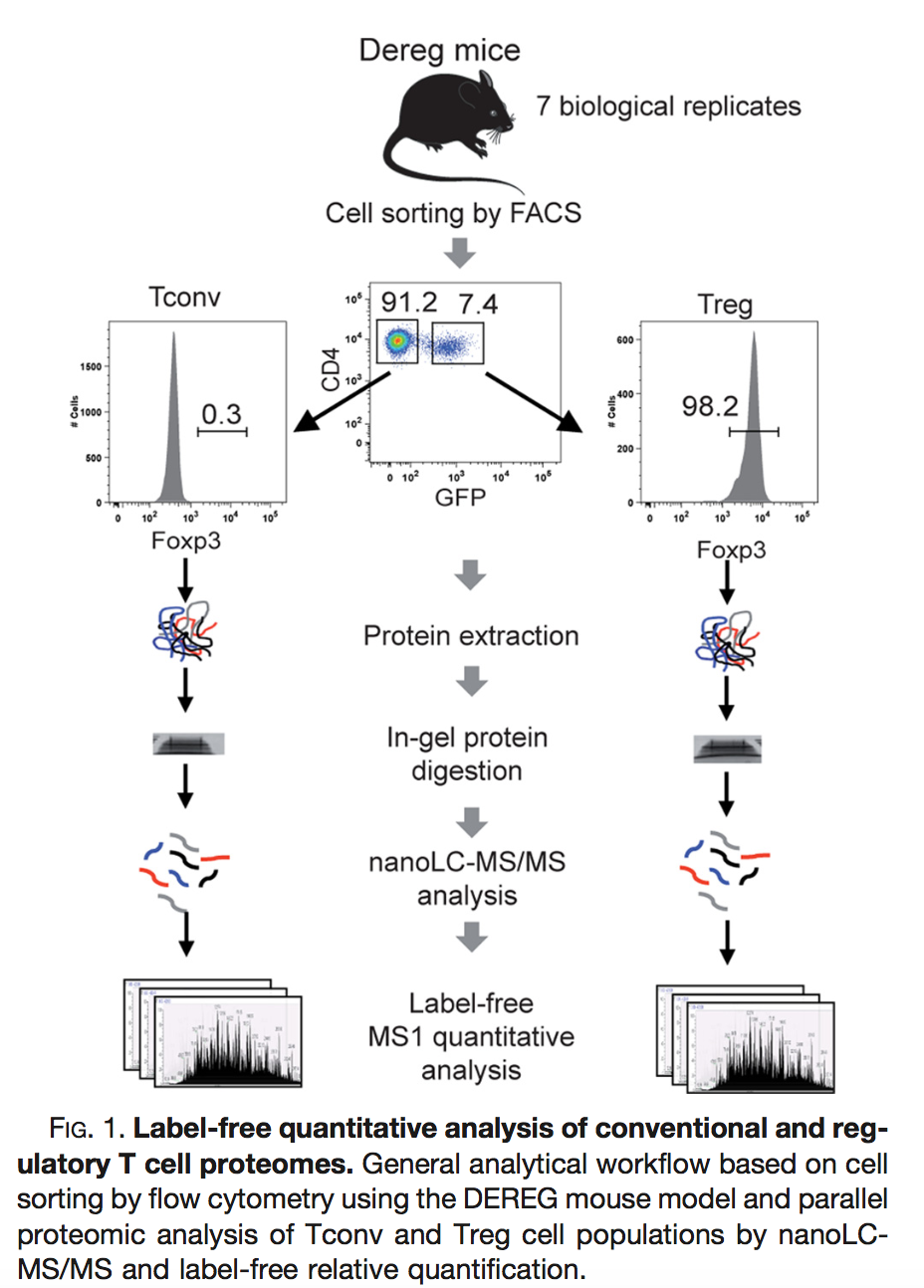
3. Blocking: Mouse T-cell example
Duguet et al. 2017 compared the proteomes of mouse regulatory T cells (Treg) and conventional T cells (Tconv) in order to discover differentially regulated proteins between these two cell populations. For each biological repeat the proteomes were extracted for both Treg and Tconv cell pools, which were purified by flow cytometry. The data in data/quantification/mouseTcell on the pdaData repository are a subset of the data PXD004436 on PRIDE.
Three subsets of the data are avialable:
- peptidesCRD.txt: contains data of Tconv cells for 4 bio-repeats and Treg cells for 4 bio-repeats
- peptidesRCB.txt: contains data for 4 bio-repeats only, but for each bio-repeat the Treg and Tconv proteome is profiled.
- peptides.txt: contains data of Treg and Tconv cells for 7 bio-repeats
Alter the cancer_3x3 script for the analysis of the Mouse T-cell example.