Visualization of Multi Dimensional Scaling (MDS) objects
Andrea Vicini
Philippe Hauchamps
Source:vignettes/MDSvis.Rmd
MDSvis.RmdAbstract
This vignette is the main one describing the functionality
implemented in the MDSvis package.
MDSvis conatins a shiny application enabling
interactive visualization of Multi Dimensional Scaling (MDS)
objects. This vignette is distributed under a CC BY-SA 4.0
license.
Installation and loading dependencies
To install this package, start R and enter:
if (!require("BiocManager", quietly = TRUE))
    install.packages("BiocManager")

if (!require("MDSvis", quietly = TRUE))
    BiocManager::install("MDSvis")
We now load the packages needed in the current vignette:
Introduction
The MDSvis package implements visualization of Multi
Dimensional Scaling (MDS) objects representing a low dimensional
projection of sample distances. Such objects can be obtained using
features implemented in the CytoMDS package (Hauchamps et al. (2025)). For more information
see the CytoMDS
vignette.
The visualization is done via a Shiny app that allows the user to
interactively customise the plots depending on a series of input
parameters (see the CytoMDS::ggplotSampleMDS() function for
more details on the parameters).
IMPORTANT: the example provided in the current
vignette uses cytometry data. As a result, the distance matrix, which
contains the pairwise sample distances, and serves as input to the MDS
projection, is here calculated from cytometry data samples using the
CytoMDS package. However, the input MDS object can also be
calculated from any distance matrix, where the units of interest are not
necessarily cytometry samples. This is demonstrated in this additional
vignette.
Illustrative dataset
We load an illustrative mass cytometry (CyTOF) dataset from (Krieg et al. 2018), accessible from the Bioconductor HDCytoData data package (Weber and Soneson (2019)).
Krieg_Anti_PD_1 was used to characterize immune cell subsets in peripheral blood from melanoma skin cancer patients treated with anti-PD-1 immunotherapy.
This study found that the frequency of CD14+CD16-HLA-DRhi monocytes in baseline samples (taken from patients prior to treatment) was a strong predictor of survival in response to immunotherapy treatment.
Notably, this dataset contains a strong batch effect, due to sample acquisition on two different days (Krieg et al. (2018)).
Generation of input files
In the current section, we show how to build the input objects needed by the shiny app, step by step. However, if you are only interested in the description of the app functionalities, you might decide to launch the application demo mode - which automatically pre-loads the Krieg_Anti_PD_1 dataset - and jump to the next section.
First we load the Krieg_Anti_PD_1 dataset, from the HDCytoData package.
Krieg_fs <- Krieg_Anti_PD_1_flowSet()## see ?HDCytoData and browseVignettes('HDCytoData') for documentation## loading from cache## Warning in updateObjectFromSlots(object, ..., verbose = verbose): dropping
## slot(s) 'colnames' from object = 'flowSet'
Krieg_fs## A flowSet with 20 experiments.
##
## column names(49): Pd104Di Pd105Di ... batch_id sample_idNext we build a phenodata dataframe with experimental design information, which are here found in the cytometry data structures.
# update phenoData structure

chLabels <-
    keyword(Krieg_fs[[1]], "MARKER_INFO")$MARKER_INFO$channel_name
chMarkers <-
    keyword(Krieg_fs[[1]], "MARKER_INFO")$MARKER_INFO$marker_name
marker_class <-
    keyword(Krieg_fs[[1]], "MARKER_INFO")$MARKER_INFO$marker_class

chLabels <- chLabels[marker_class != "none"]
chMarkers <- chMarkers[marker_class != "none"]
# marker_class all equal to "type", 24 markers are left

phenoData <- flowCore::pData(Krieg_fs)
additionalPhenoData <-
    keyword(Krieg_fs[[1]], "EXPERIMENT_INFO")$EXPERIMENT_INFO
phenoData <- cbind(phenoData, additionalPhenoData)

flowCore::pData(Krieg_fs) <- phenoData
Next, we scale-transform the mass cytometry data and calculate the pairwise distance matrix.
# transform flow set (arcsinh(cofactor = 5))
trans <- arcsinhTransform(
    transformationId="ArcsinhTransform",
    a = 0,
    b = 1/5,
    c = 0)

# Applying arcsinh() transformation
Krieg_fs_trans <- transform(
    Krieg_fs,
    transformList(chLabels, trans))

# Calculating Sample distances
pwDist <- pairwiseEMDDist(
    Krieg_fs_trans,
    channels = chMarkers,
    verbose = FALSE
)
From the distance matrix, we can now calculate the MDS projection.
This is also done using the CytoMDS package.
mdsObj <- computeMetricMDS(
    pwDist,
    seed = 0)

show(mdsObj)
## MDS object containing MDS projection (using Smacof algorithm) data:
## Nb of dimensions: 2
## Nb of points: 20
## Stress: 0.052363
## Pseudo RSquare: 0.984008
## Goodness of fit: 0.997258Optionally, for the use of biplots as an interpretation tool, sample
specific statistics can be provided by the user. Here we calculate
standard univariate statistics from each variable of the
multidimensional distribution (again using the CytoMDS
package).
# Computing sample statistics

statFUNs <- c(
    "median" = stats::median,
    "std-dev" = stats::sd,
    "mean" = base::mean,
    "Q25" = function(x, na.rm)
        stats::quantile(x, probs = 0.25, na.rm = na.rm),
    "Q75" = function(x, na.rm)
        stats::quantile(x, probs = 0.75, na.rm = na.rm))

chStats <- CytoMDS::channelSummaryStats(
    Krieg_fs_trans,
    channels = chMarkers,
    statFUNs = statFUNs)
The newly created objects can be saved as .rds files.
These files can in turn be selected within the shiny app for
visualization.
Visualization of the MDS projection
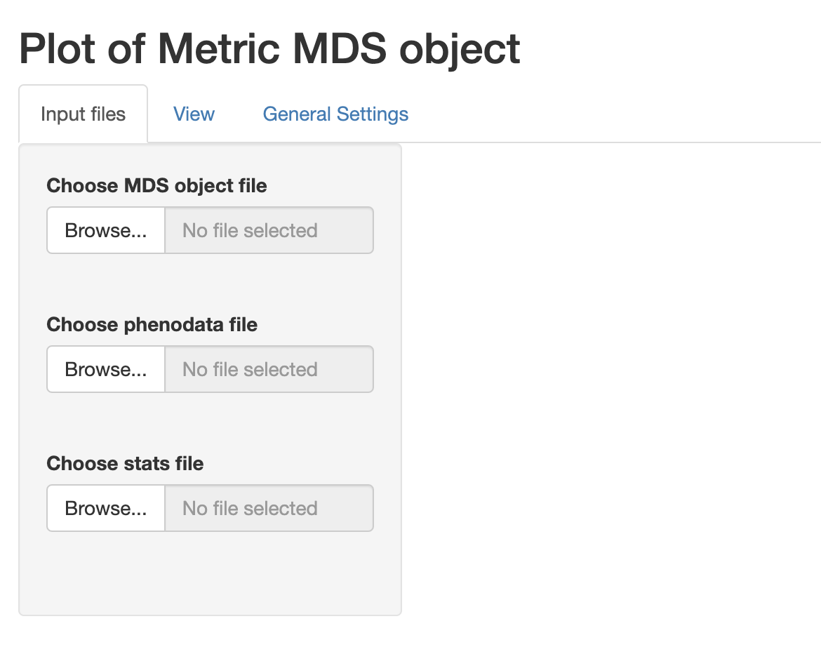
The MDSvis function run_app launches the
interactive Shiny app and the three tabs window in the figure below gets
opened.
MDSvis::mdsvis_app()

# alternatively launch the application in demo mode, with the Krieg_Anti_PD_1
# dataset already loaded.
#MDSvis::mdsvis_app(preLoadDemoDataset = TRUE)
In the ‘Input files’ tab the objects can be loaded for visualization. The plots are then shown in the ‘View’ tab while the ‘General settings’ contains more technical plot settings controls. All the input files are expected to have .rds extension and at least a file containing the MDS object has to be loaded. Optionally a phenodata file containing a phenodata dataframe and/or a file containing a list of statistics for biplot visualization can be loaded.
Alternatively, a ‘demo mode’ (see in commented code chunck above) allows the user to launch the app with the Krieg_Anti_PD_1 dataset pre-loaded, without importing input .rds files.
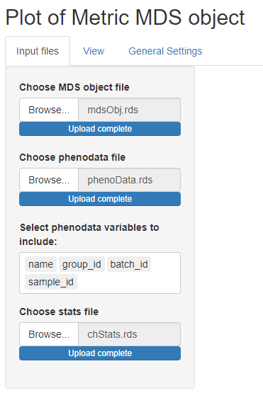
 We can select the previously
created files and proceed with the visualization. Note that when a
phenodata file is selected a new control appears allowing to select only
a subset of variables (by default all are selected). These phenodata
selected variables will be the only ones available in the drop-down list
controls in the ‘View’ tab.
We can select the previously
created files and proceed with the visualization. Note that when a
phenodata file is selected a new control appears allowing to select only
a subset of variables (by default all are selected). These phenodata
selected variables will be the only ones available in the drop-down list
controls in the ‘View’ tab.
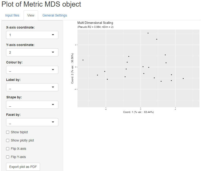
 We can now open the ‘View’ tab
to see the plot of the projection results. The controls on the side
allow to choose the projection axes; colour, label, define facet or
shape the points according to phenodata variables; add biplot; show a
We can now open the ‘View’ tab
to see the plot of the projection results. The controls on the side
allow to choose the projection axes; colour, label, define facet or
shape the points according to phenodata variables; add biplot; show a
plotly plot for interactive plot exploration or flip
axes.
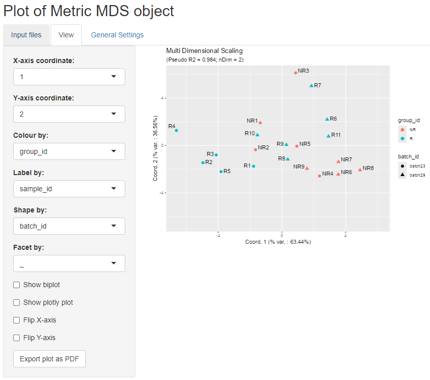
 For example we can colour the points
according to group_id, label the points according to sample_id, and use
shapes according to batch_id, as shown in the figure below.
For example we can colour the points
according to group_id, label the points according to sample_id, and use
shapes according to batch_id, as shown in the figure below.
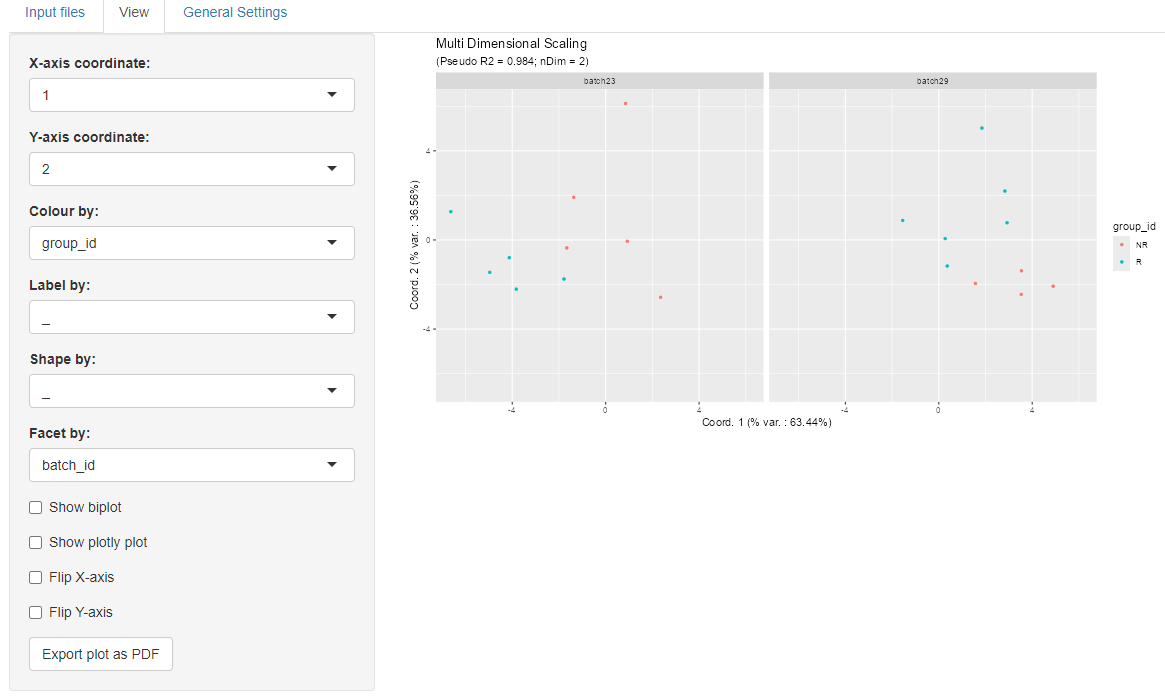
 We can also defne facets according to
the two batches, as in the figure below:
We can also defne facets according to
the two batches, as in the figure below:
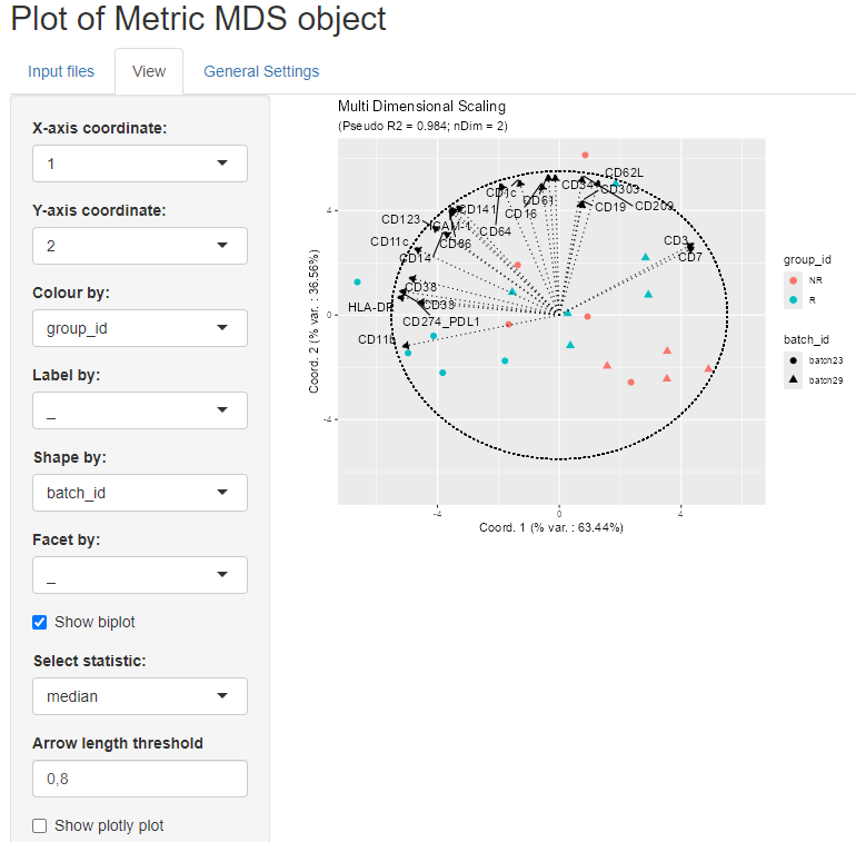
We can also add a biplot created based on sample statistics by clicking on the biplot checkbox. The idea is to calculate the correlation of the sample statistics w.r.t. the axes of projection, so that these correlations can be represented on a correlation circle overlaid on the projection plot.
The desired statistic can be selected from the drop down menu and it
is possible to show only the arrows that respect a selected length
threshold.
In the example below, the chosen statistic is the median while the arrow
length threshold is 0.8.
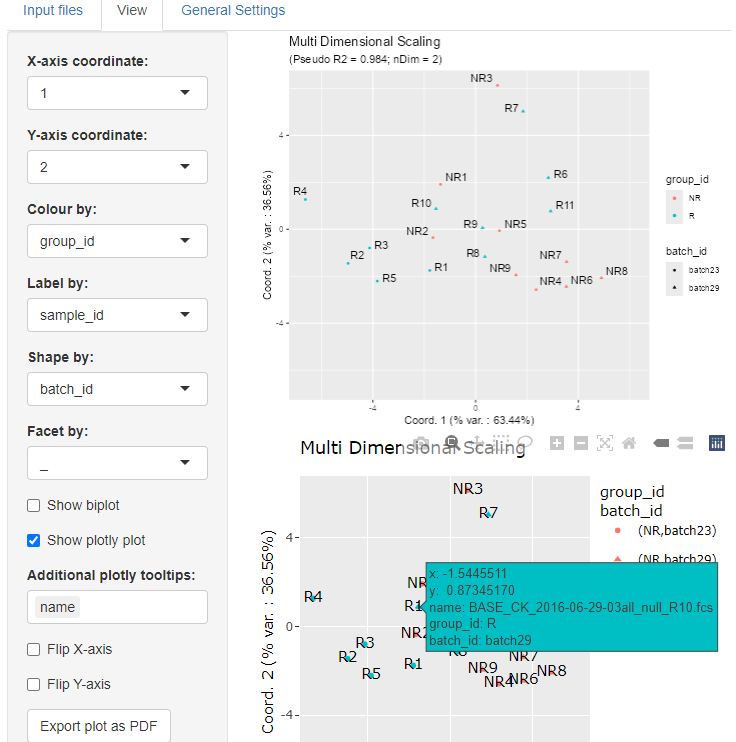
When some data are too large to be displayed as labels, one possible
solution is to display an interactive plotly plot below the
regular one by selecting the corresponding checkbox.
We can add new plotly tooltips and highlight the
corresponding information for each point by hovering over them.
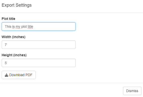
Finally, the obtained plots can be exported as a pdf file. The user can defined the corresponding plot title, pdf file name and plot size (with and height) to be used.
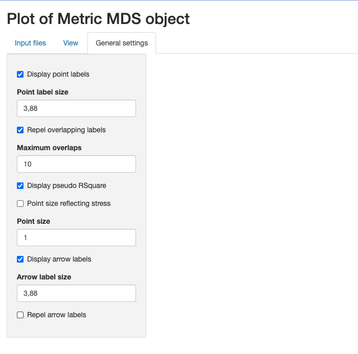
General settings
For completeness we show below the ‘General settings’ tab which
contains some general controls regarding e.g. points features, the
corresponding labels and biplot arrows. For more details see the
CytoMDS::ggplotSampleMDS() function parameters.
Session information
## R Under development (unstable) (2026-01-10 r89298)
## Platform: x86_64-pc-linux-gnu
## Running under: Ubuntu 24.04.3 LTS
##
## Matrix products: default
## BLAS:   /usr/lib/x86_64-linux-gnu/openblas-pthread/libblas.so.3
## LAPACK: /usr/lib/x86_64-linux-gnu/openblas-pthread/libopenblasp-r0.3.26.so;  LAPACK version 3.12.0
##
## locale:
##  [1] LC_CTYPE=en_US.UTF-8       LC_NUMERIC=C
##  [3] LC_TIME=en_US.UTF-8        LC_COLLATE=en_US.UTF-8
##  [5] LC_MONETARY=en_US.UTF-8    LC_MESSAGES=en_US.UTF-8
##  [7] LC_PAPER=en_US.UTF-8       LC_NAME=C
##  [9] LC_ADDRESS=C               LC_TELEPHONE=C
## [11] LC_MEASUREMENT=en_US.UTF-8 LC_IDENTIFICATION=C
##
## time zone: UTC
## tzcode source: system (glibc)
##
## attached base packages:
## [1] stats4    stats     graphics  grDevices utils     datasets  methods
## [8] base
##
## other attached packages:
##  [1] MDSvis_0.99.6               CytoMDS_1.7.1
##  [3] HDCytoData_1.31.0           flowCore_2.23.1
##  [5] SummarizedExperiment_1.41.0 Biobase_2.71.0
##  [7] GenomicRanges_1.63.1        Seqinfo_1.1.0
##  [9] IRanges_2.45.0              S4Vectors_0.49.0
## [11] MatrixGenerics_1.23.0       matrixStats_1.5.0
## [13] ExperimentHub_3.1.0         AnnotationHub_4.1.0
## [15] BiocFileCache_3.1.0         dbplyr_2.5.1
## [17] BiocGenerics_0.57.0         generics_0.1.4
## [19] BiocStyle_2.39.0
##
## loaded via a namespace (and not attached):
##   [1] splines_4.6.0        later_1.4.5          filelock_1.0.3
##   [4] tibble_3.3.1         graph_1.89.1         XML_3.99-0.20
##   [7] rpart_4.1.24         lifecycle_1.0.5      httr2_1.2.2
##  [10] Rdpack_2.6.4         doParallel_1.0.17    flowWorkspace_4.23.1
##  [13] lattice_0.22-7       MASS_7.3-65          backports_1.5.0
##  [16] magrittr_2.0.4       Hmisc_5.2-5          plotly_4.11.0
##  [19] sass_0.4.10          rmarkdown_2.30       plotrix_3.8-13
##  [22] jquerylib_0.1.4      yaml_2.3.12          httpuv_1.6.16
##  [25] otel_0.2.0           DBI_1.2.3            minqa_1.2.8
##  [28] RColorBrewer_1.1-3   abind_1.4-8          ggcyto_1.39.1
##  [31] purrr_1.2.1          nnet_7.3-20          pracma_2.4.6
##  [34] rappdirs_0.3.3       transport_0.15-4     gdata_3.0.1
##  [37] ellipse_0.5.0        pkgdown_2.2.0.9000   codetools_0.2-20
##  [40] DelayedArray_0.37.0  tidyselect_1.2.1     shape_1.4.6.1
##  [43] farver_2.1.2         lme4_1.1-38          base64enc_0.1-3
##  [46] jsonlite_2.0.0       e1071_1.7-17         mitml_0.4-5
##  [49] Formula_1.2-5        survival_3.8-3       iterators_1.0.14
##  [52] systemfonts_1.3.1    foreach_1.5.2        tools_4.6.0
##  [55] ragg_1.5.0           Rcpp_1.1.1           glue_1.8.0
##  [58] gridExtra_2.3        pan_1.9              SparseArray_1.11.10
##  [61] xfun_0.55            dplyr_1.1.4          withr_3.0.2
##  [64] BiocManager_1.30.27  fastmap_1.2.0        boot_1.3-32
##  [67] shinyjs_2.1.1        digest_0.6.39        R6_2.6.1
##  [70] mime_0.13            mice_3.19.0          textshaping_1.0.4
##  [73] colorspace_2.1-2     gtools_3.9.5         RSQLite_2.4.5
##  [76] weights_1.1.2        tidyr_1.3.2          hexbin_1.28.5
##  [79] data.table_1.18.0    class_7.3-23         httr_1.4.7
##  [82] htmlwidgets_1.6.4    S4Arrays_1.11.1      pkgconfig_2.0.3
##  [85] gtable_0.3.6         blob_1.3.0           RProtoBufLib_2.23.0
##  [88] S7_0.2.1             XVector_0.51.0       htmltools_0.5.9
##  [91] bookdown_0.46        scales_1.4.0         png_0.1-8
##  [94] wordcloud_2.6        reformulas_0.4.3.1   knitr_1.51
##  [97] rstudioapi_0.17.1    checkmate_2.3.3      nlme_3.1-168
## [100] curl_7.0.0           nloptr_2.2.1         proxy_0.4-29
## [103] cachem_1.1.0         stringr_1.6.0        BiocVersion_3.23.1
## [106] parallel_4.6.0       foreign_0.8-90       AnnotationDbi_1.73.0
## [109] desc_1.4.3           pillar_1.11.1        grid_4.6.0
## [112] vctrs_0.6.5          promises_1.5.0       cytolib_2.23.0
## [115] jomo_2.7-6           xtable_1.8-4         cluster_2.1.8.1
## [118] htmlTable_2.4.3      Rgraphviz_2.55.0     evaluate_1.0.5
## [121] cli_3.6.5            compiler_4.6.0       rlang_1.1.7
## [124] crayon_1.5.3         smacof_2.1-7         ncdfFlow_2.57.0
## [127] plyr_1.8.9           fs_1.6.6             stringi_1.8.7
## [130] viridisLite_0.4.2    BiocParallel_1.45.0  nnls_1.6
## [133] Biostrings_2.79.4    lazyeval_0.2.2       glmnet_4.1-10
## [136] Matrix_1.7-4         bit64_4.6.0-1        CytoPipeline_1.11.0
## [139] ggplot2_4.0.1        KEGGREST_1.51.1      shiny_1.12.1
## [142] rbibutils_2.4        broom_1.0.11         memoise_2.0.1
## [145] bslib_0.9.0          bit_4.6.0            polynom_1.4-1