Load Single-Cell Proteomics data using readSCP

Laurent Gatto

Christophe Vanderaa

31 May 2025

The scp data framework

Our data structure is relying on three curated data classes: QFeatures (Gatto and Vanderaa (2023)),SummarizedExperiment and SingleCellExperiment (Amezquita et al. (2020)). QFeatures is dedicated to the manipulation and processing of MS-based quantitative data. It explicitly records the successive steps to allow users to navigate up and down the different MS levels. SummarizedExperiment is a class designed to store and manipulate quantitative data. Its the base building block of a QFeatures object. SingleCellExperiment is another class designed as an efficient data container that serves as an interface to state-of-the-art methods and algorithms for single-cell data. This class is used in the context of data modeling (scplainer).

Our framework combines the three classes to inherit from their respective advantages.

Because mass spectrometry (MS)-based single-cell proteomics (SCP) only captures the proteome of between one and a few tens of single-cells in a single run, the data is usually acquired across many MS batches. Therefore, the data for each run should conceptually be stored in its own container, that we here call a set. The expected input for working with the scp package is quantification data of peptide to spectrum matches (PSM). These data can then be processed to reconstruct peptide and protein data. The links between related features across different sets are stored to facilitate manipulation and visualization of of PSM, peptide and protein data. This is conceptually shown below.

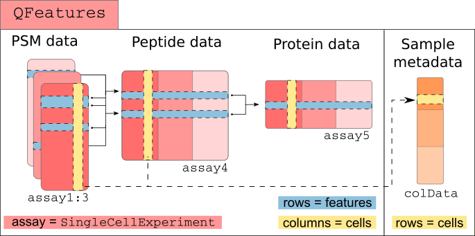
The scp framework relies on SingleCellExperiment and QFeatures objects

The main input table required for starting an analysis with scp is called the assayData.

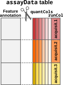
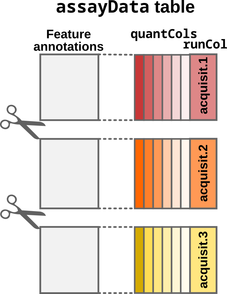
assayData table

The assayData table is generated after the identification and quantification of the MS spectra by a pre-processing software such as MaxQuant, ProteomeDiscoverer or MSFragger (the list of available software is actually much longer). We will here use as an example a data table that has been generated by MaxQuant. The table is available from the scp package and is called mqScpData (for MaxQuant generated SCP data).

library(scp)
data("mqScpData")
dim(mqScpData)
#> [1] 1361  149

In this toy example, there are 1361 rows corresponding to features (quantified PSMs) and 149 columns corresponding to different data fields recorded by MaxQuant during the processing of the MS spectra. There are three types of columns:

• Quantification columns (quantCols): 1 to n (depending on technology)
• Run identifier column (runCol): e.g. file name
• Feature annotations: e.g. peptide sequence, ion charge, protein name

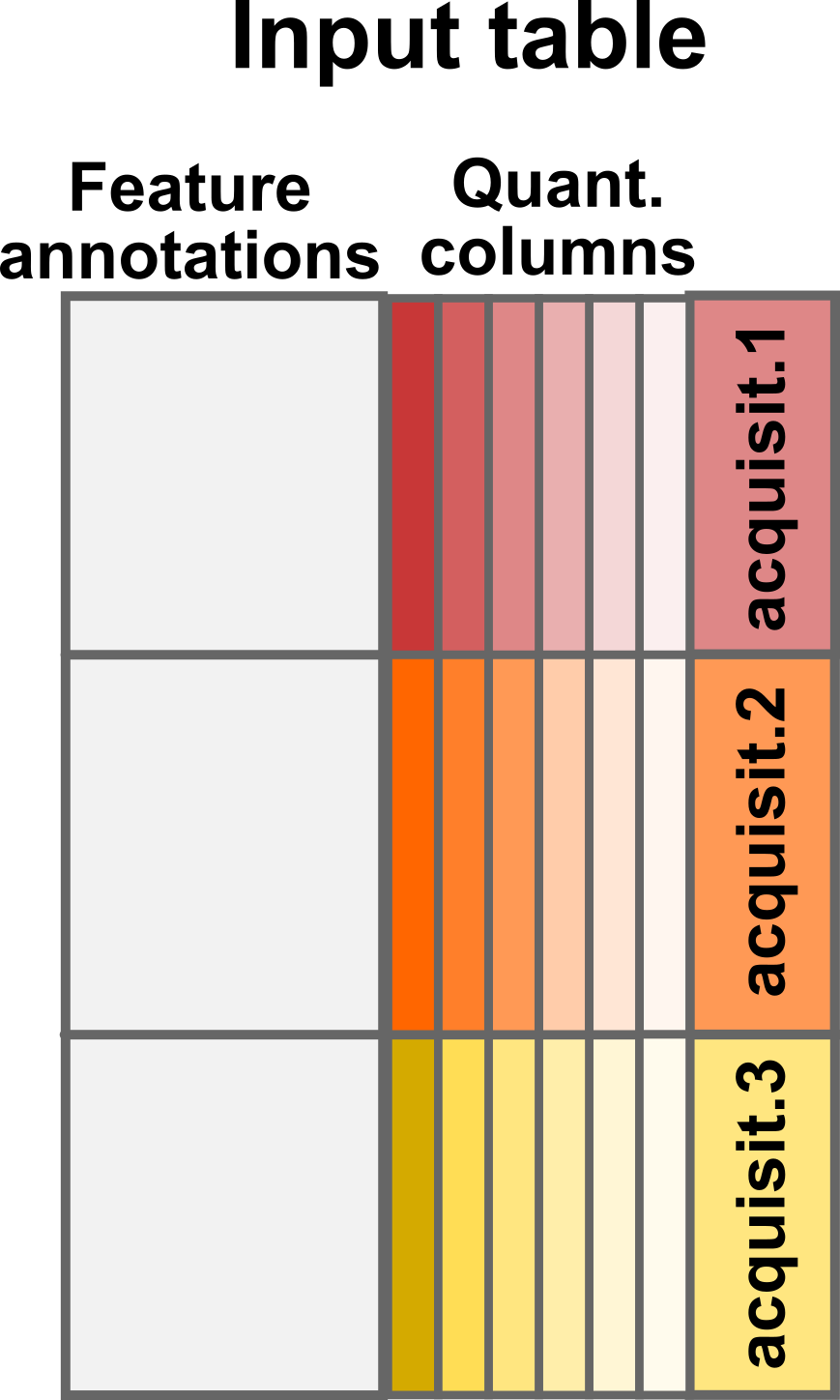
Conceptual representation of the assayData input table

Quantification columns (quantCols)

The quantification data can be composed of one (in case of label-free acquisition) or multiple columns (in case of multiplexing). In the example data set, the columns holding the quantification, the quantCols, start with Reporter.intensity. followed by a number.

(quantCols <- grep("Reporter.intensity.\\d", colnames(mqScpData),
                  value = TRUE))
#>  [1] "Reporter.intensity.1"  "Reporter.intensity.2"  "Reporter.intensity.3" 
#>  [4] "Reporter.intensity.4"  "Reporter.intensity.5"  "Reporter.intensity.6" 
#>  [7] "Reporter.intensity.7"  "Reporter.intensity.8"  "Reporter.intensity.9" 
#> [10] "Reporter.intensity.10" "Reporter.intensity.11" "Reporter.intensity.12"
#> [13] "Reporter.intensity.13" "Reporter.intensity.14" "Reporter.intensity.15"
#> [16] "Reporter.intensity.16"

As you may notice, the example data was acquired using a TMT-16 protocol since we retrieve 16 quantification columns. Actually, some runs were acquired using a TMT-11 protocol (11 labels) but we will come back to this later.

head(mqScpData[, quantCols])
#>   Reporter.intensity.1 Reporter.intensity.2 Reporter.intensity.3
#> 1                61251               501.71               3731.3
#> 2                58648              1099.80               2837.7
#> 3               150350              3705.00               9361.0
#> 4                27347               405.90               1525.2
#> 5                84035               583.09               4092.3
#> 6                44895               700.23               2283.0
#>   Reporter.intensity.4 Reporter.intensity.5 Reporter.intensity.6
#> 1              1643.30               871.84               981.87
#> 2               494.32               349.26              1030.50
#> 3                 0.00              1945.40              1188.60
#> 4                 0.00                 0.00               318.74
#> 5               530.13               718.13              2204.50
#> 6              1109.60                 0.00               675.79
#>   Reporter.intensity.7 Reporter.intensity.8 Reporter.intensity.9
#> 1              1200.10               939.06              1457.50
#> 2                 0.00              1214.10               800.58
#> 3              1574.00              2302.10              2176.10
#> 4                 0.00               519.81                 0.00
#> 5               960.51               453.77              1188.40
#> 6                 0.00               809.38               668.88
#>   Reporter.intensity.10 Reporter.intensity.11 Reporter.intensity.12
#> 1               1329.80                981.83                    NA
#> 2                807.79                391.38                    NA
#> 3               1399.50               1307.50                2192.4
#> 4                507.23                370.79                    NA
#> 5                740.99                  0.00                    NA
#> 6               1467.50                901.38                    NA
#>   Reporter.intensity.13 Reporter.intensity.14 Reporter.intensity.15
#> 1                    NA                    NA                    NA
#> 2                    NA                    NA                    NA
#> 3                1791.4                1727.5                2157.3
#> 4                    NA                    NA                    NA
#> 5                    NA                    NA                    NA
#> 6                    NA                    NA                    NA
#>   Reporter.intensity.16
#> 1                    NA
#> 2                    NA
#> 3                  1398
#> 4                    NA
#> 5                    NA
#> 6                    NA

Run identifier column (runCol)

This column provides the identifier of the MS runs in which each PSM was acquired. MaxQuant uses the raw file name to identify the run.

unique(mqScpData$Raw.file)
#> [1] "190321S_LCA10_X_FP97AG"        "190222S_LCA9_X_FP94BM"        
#> [3] "190914S_LCB3_X_16plex_Set_21"  "190321S_LCA10_X_FP97_blank_01"

Feature annotations

The remaining columns in the mqScpData table contain information used or generated during the identification of the MS spectra. For instance, you may find the charge of the parent ion, the score and probability of a correct match between the MS spectrum and a peptide sequence, the sequence of the best matching peptide, its length, its modifications, the retention time of the peptide on the LC, the protein(s) the peptide originates from and much more.

head(mqScpData[, c("Charge", "Score", "PEP", "Sequence", "Length",
                   "Retention.time", "Proteins")])
#>   Charge  Score        PEP    Sequence Length Retention.time
#> 1      2 41.029 5.2636e-04   ATNFLAHEK      9         65.781
#> 2      2 44.349 5.8789e-04   ATNFLAHEK      9         63.787
#> 3      2 51.066 4.0315e-24 SHTILLVQPTK     11         71.884
#> 4      2 63.816 4.7622e-06 SHTILLVQPTK     11         68.633
#> 5      2 74.464 6.8709e-09 SHTILLVQPTK     11         71.946
#> 6      2 41.502 5.3705e-02     SLVIPEK      7         76.204
#>               Proteins
#> 1 sp|P29692|EF1D_HUMAN
#> 2 sp|P29692|EF1D_HUMAN
#> 3  sp|P84090|ERH_HUMAN
#> 4  sp|P84090|ERH_HUMAN
#> 5  sp|P84090|ERH_HUMAN
#> 6 sp|P62269|RS18_HUMAN

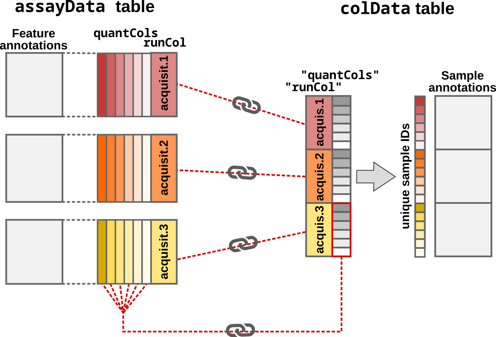
colData table

The colData table contains the experimental design generated by the researcher. The rows of the sample table correspond to a sample in the experiment and the columns correspond to the available annotations about the sample. We will here use the second example table:

data("sampleAnnotation")
head(sampleAnnotation)
#>                  runCol            quantCols SampleType lcbatch sortday digest
#> 1 190222S_LCA9_X_FP94BM Reporter.intensity.1    Carrier    LCA9      s8      N
#> 2 190222S_LCA9_X_FP94BM Reporter.intensity.2  Reference    LCA9      s8      N
#> 3 190222S_LCA9_X_FP94BM Reporter.intensity.3     Unused    LCA9      s8      N
#> 4 190222S_LCA9_X_FP94BM Reporter.intensity.4   Monocyte    LCA9      s8      N
#> 5 190222S_LCA9_X_FP94BM Reporter.intensity.5      Blank    LCA9      s8      N
#> 6 190222S_LCA9_X_FP94BM Reporter.intensity.6   Monocyte    LCA9      s8      N

The colData table may contain any information about the samples. For example, useful information could be the type of sample that is analysed, a phenotype known from the experimental design, the MS batch, the acquisition date, MS settings used to acquire the sample, the LC batch, the sample preparation batch, etc… However, scp requires 2 specific columns in the colData table:

1. runCol: this column provides the MS run names (that match the Raw.file column in the assayData table).
2. quantCols: this column tells scp the names of the columns in the feature data holds the quantification of the corresponding sample.

These two columns allow scp to correctly split and match data that were acquired across multiple acquisition runs.

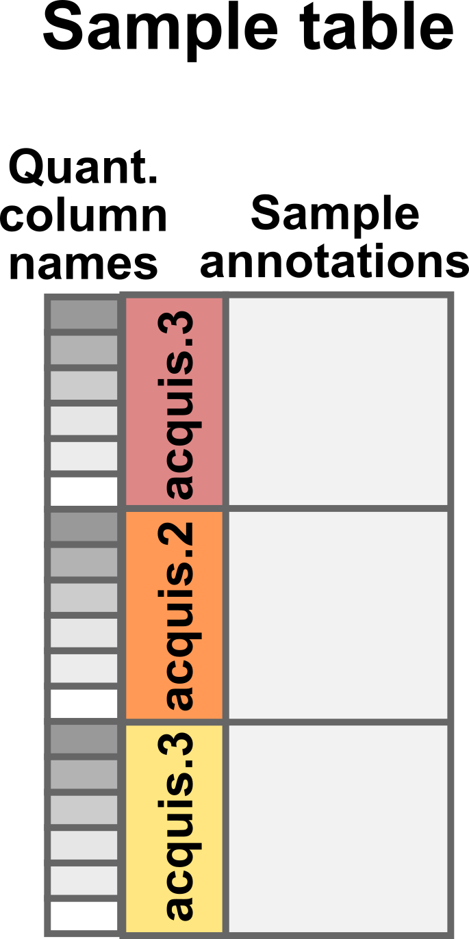
Conceptual representation of the sample table

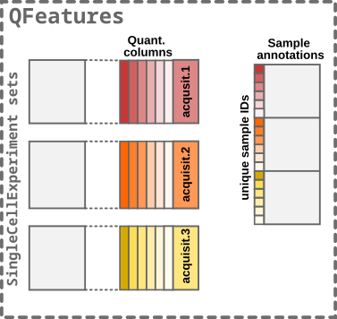
readSCP()

readSCP is the function that converts the assayData and the colData into a QFeatures object following the data structure described above, that is storing the data belonging to each MS batch in a separate SingleCellExperiment object.

Sample names

readSCP() automatically assigns names that are unique across all samples in all sets. This is performed by appending the name of the MS run where a given sample is found with the name of the quantification column for that sample. Suppose a sample belongs to batch 190222S_LCA9_X_FP94BM and the quantification values in the assayData table are found in the column called Reporter.intensity.3, then the sample name will become 190222S_LCA9_X_FP94BM_Reporter.intensity.3.

Special case: empty samples

In some rare cases, it can be beneficial to remove empty samples (all quantifications are NA) from the sets. Such samples can occur when samples that were acquired with different multiplexing labels are merged in a single table. For instance, the SCoPE2 data we provide as an example contains runs that were acquired with two TMT protocols. The 3 first sets were acquired using the TMT-11 protocol and the last set was acquired using a TMT-16 protocol. The missing label channels in the TMT-11 data are filled with NAs. When setting removeEmptyCols = TRUE, readSCP() automatically detects and removes columns containing only NAs,

Running readSCP

We convert the sample and the feature data into a QFeatures object in a single command thanks to readSCP.

(scp <- readSCP(assayData = mqScpData,
                colData = sampleAnnotation,
                runCol = "Raw.file",
                removeEmptyCols = TRUE))
#> Checking arguments.
#> Loading data as a 'SummarizedExperiment' object.
#> Splitting data in runs.
#> Formatting sample annotations (colData).
#> Formatting data as a 'QFeatures' object.
#> An instance of class QFeatures (type: scp) with 4 sets:
#> 
#>  [1] 190222S_LCA9_X_FP94BM: SummarizedExperiment with 395 rows and 11 columns 
#>  [2] 190321S_LCA10_X_FP97_blank_01: SummarizedExperiment with 109 rows and 11 columns 
#>  [3] 190321S_LCA10_X_FP97AG: SummarizedExperiment with 487 rows and 11 columns 
#>  [4] 190914S_LCB3_X_16plex_Set_21: SummarizedExperiment with 370 rows and 16 columns

The object returned by readSCP() is a QFeatures object containing 4 SingleCellExperiment sets that have been named after the 4 MS batches. Each set contains either 11 or 16 columns (samples) depending on the TMT labelling strategy and a variable number of rows (quantified PSMs). Each piece of information can easily be retrieved thanks to the QFeatures architectures. As mentioned in another vignette, the colData is retrieved using its dedicated function:

head(colData(scp))
#> DataFrame with 6 rows and 6 columns
#>                                                   runCol     quantCols
#>                                              <character>   <character>
#> 190222S_LCA9_X_FP94BM_Reporter.intensity.1 190222S_LC... Reporter.i...
#> 190222S_LCA9_X_FP94BM_Reporter.intensity.2 190222S_LC... Reporter.i...
#> 190222S_LCA9_X_FP94BM_Reporter.intensity.3 190222S_LC... Reporter.i...
#> 190222S_LCA9_X_FP94BM_Reporter.intensity.4 190222S_LC... Reporter.i...
#> 190222S_LCA9_X_FP94BM_Reporter.intensity.5 190222S_LC... Reporter.i...
#> 190222S_LCA9_X_FP94BM_Reporter.intensity.6 190222S_LC... Reporter.i...
#>                                             SampleType     lcbatch     sortday
#>                                            <character> <character> <character>
#> 190222S_LCA9_X_FP94BM_Reporter.intensity.1     Carrier        LCA9          s8
#> 190222S_LCA9_X_FP94BM_Reporter.intensity.2   Reference        LCA9          s8
#> 190222S_LCA9_X_FP94BM_Reporter.intensity.3      Unused        LCA9          s8
#> 190222S_LCA9_X_FP94BM_Reporter.intensity.4    Monocyte        LCA9          s8
#> 190222S_LCA9_X_FP94BM_Reporter.intensity.5       Blank        LCA9          s8
#> 190222S_LCA9_X_FP94BM_Reporter.intensity.6    Monocyte        LCA9          s8
#>                                                 digest
#>                                            <character>
#> 190222S_LCA9_X_FP94BM_Reporter.intensity.1           N
#> 190222S_LCA9_X_FP94BM_Reporter.intensity.2           N
#> 190222S_LCA9_X_FP94BM_Reporter.intensity.3           N
#> 190222S_LCA9_X_FP94BM_Reporter.intensity.4           N
#> 190222S_LCA9_X_FP94BM_Reporter.intensity.5           N
#> 190222S_LCA9_X_FP94BM_Reporter.intensity.6           N

The feature annotations are retrieved from the rowData. Since the feature annotations are specific to each set, we need to tell from which set we want to get the rowData:

head(rowData(scp[["190222S_LCA9_X_FP94BM"]]))[, 1:5]
#> DataFrame with 6 rows and 5 columns
#>              uid      Sequence    Length Modifications Modified.sequence
#>      <character>   <character> <integer>   <character>       <character>
#> 2  _(Acetyl (...     ATNFLAHEK         9 Acetyl (Pr...     _(Acetyl (...
#> 4  _(Acetyl (... SHTILLVQPT...        11 Acetyl (Pr...     _(Acetyl (...
#> 6  _(Acetyl (...       SLVIPEK         7 Acetyl (Pr...     _(Acetyl (...
#> 9  _AAGLALK_ ...       AAGLALK         7    Unmodified         _AAGLALK_
#> 12 _AALSAGK_ ...       AALSAGK         7    Unmodified         _AALSAGK_
#> 15 _AAPEASGTP... AAPEASGTPS...        16    Unmodified     _AAPEASGTP...

Finally, we can also retrieve the quantification matrix for a set of interest:

head(assay(scp, "190222S_LCA9_X_FP94BM"))
#>    190222S_LCA9_X_FP94BM_Reporter.intensity.1
#> 2                                     58648.0
#> 4                                     27347.0
#> 6                                     44895.0
#> 9                                    122070.0
#> 12                                    58605.0
#> 15                                     5006.5
#>    190222S_LCA9_X_FP94BM_Reporter.intensity.2
#> 2                                     1099.80
#> 4                                      405.90
#> 6                                      700.23
#> 9                                     1153.50
#> 12                                     895.25
#> 15                                     517.86
#>    190222S_LCA9_X_FP94BM_Reporter.intensity.3
#> 2                                     2837.70
#> 4                                     1525.20
#> 6                                     2283.00
#> 9                                     7361.90
#> 12                                    2763.80
#> 15                                     446.19
#>    190222S_LCA9_X_FP94BM_Reporter.intensity.4
#> 2                                      494.32
#> 4                                        0.00
#> 6                                     1109.60
#> 9                                     1732.30
#> 12                                     867.82
#> 15                                     458.17
#>    190222S_LCA9_X_FP94BM_Reporter.intensity.5
#> 2                                      349.26
#> 4                                        0.00
#> 6                                        0.00
#> 9                                     1515.60
#> 12                                    1050.30
#> 15                                     467.90
#>    190222S_LCA9_X_FP94BM_Reporter.intensity.6
#> 2                                     1030.50
#> 4                                      318.74
#> 6                                      675.79
#> 9                                     2252.00
#> 12                                    1268.70
#> 15                                     649.50
#>    190222S_LCA9_X_FP94BM_Reporter.intensity.7
#> 2                                        0.00
#> 4                                        0.00
#> 6                                        0.00
#> 9                                      444.48
#> 12                                     532.30
#> 15                                     259.84
#>    190222S_LCA9_X_FP94BM_Reporter.intensity.8
#> 2                                     1214.10
#> 4                                      519.81
#> 6                                      809.38
#> 9                                     2343.80
#> 12                                    1073.10
#> 15                                     533.55
#>    190222S_LCA9_X_FP94BM_Reporter.intensity.9
#> 2                                      800.58
#> 4                                        0.00
#> 6                                      668.88
#> 9                                     3100.20
#> 12                                     911.30
#> 15                                     393.53
#>    190222S_LCA9_X_FP94BM_Reporter.intensity.10
#> 2                                       807.79
#> 4                                       507.23
#> 6                                      1467.50
#> 9                                      1825.20
#> 12                                     1300.00
#> 15                                      463.26
#>    190222S_LCA9_X_FP94BM_Reporter.intensity.11
#> 2                                       391.38
#> 4                                       370.79
#> 6                                       901.38
#> 9                                      2372.50
#> 12                                     1185.90
#> 15                                      353.04

Under the hood

readSCP proceeds as follows:

1. The assayData table must be provided as a data.frame. readSCP() converts the table to a SingleCellExperiment object but it needs to know which column(s) store the quantitative data. Those column name(s) is/are provided by the quantCols field in the annotation table (colData argument).

Step1: Convert the input table to a SingleCellExperiment object

2. The SingleCellExperiment object is then split according to the acquisition run. The split is performed depending on the runCol field in assayData. It is also indicated in the runCol argument. In this case, the data will be split according to the Raw.file column in mqScpData. Raw.file contains the names of the acquisition runs that was used by MaxQuant to retrieve the raw data files.

Step2: Split by acquisition run

3. The sample annotations is generated from the supplied sample table (colData argument). Note that in order for readSCP() to correctly match the feature data with the annotations, colData must contain a runCol column with run names and a quantCols column with the names of the quantitative columns in assayData.

Step3: Adding and matching the sample annotations

4. Finally, the SingleCellExperiment sets and the colData are converted to a QFeatures object.

Step4: Converting to a QFeatures

What about label-free SCP?

The scp package is meant for both label-free and multiplexed SCP data. Like in the example above, the label-free data should contain the batch names in both the feature data and the sample data. The sample data must also contain a column that points to the columns of the feature data that contains the quantifications. Since label-free SCP acquires one single-cell per run, this sample data column should point the same column for all samples. Moreover, this means that each PSM set will contain a single column.

What about other input formats?

readSCP() should work with any PSM quantification table that is output by a pre-processing software. For instance, you can easily import the PSM tables generated by ProteomeDiscoverer. The batch names are contained in the File ID column (that should be supplied as the batchCol argument to readSCP()). The quantification columns are contained in the columns starting with Abundance, eventually followed by a multiplexing tag name. These columns should be stored in a dedicated column of the sample data to be supplied as runCol to readSCP().

If your input cannot be loaded using the procedure described in this vignette, you can submit a feature request (see next section).

The readSCPfromDIANN() function is adapted to import label-free and plexDIA/mTRAQ Report.tsv files generated by DIA-NN.

For more information, see the readQFeatures() and readQFeaturesFromDIANN() manual pages, that described the main principle that concern the data import and formatting.

Need help?

You can open an issue on the GitHub repository in case of troubles when loading your SCP data with readSCP(). Any suggestion or feature request about the function or the documentation are also warmly welcome.

Session information

R version 4.5.0 (2025-04-11)
Platform: x86_64-pc-linux-gnu
Running under: Ubuntu 24.04.2 LTS

Matrix products: default
BLAS:   /usr/lib/x86_64-linux-gnu/openblas-pthread/libblas.so.3 
LAPACK: /usr/lib/x86_64-linux-gnu/openblas-pthread/libopenblasp-r0.3.26.so;  LAPACK version 3.12.0

locale:
 [1] LC_CTYPE=en_US.UTF-8       LC_NUMERIC=C              
 [3] LC_TIME=en_US.UTF-8        LC_COLLATE=en_US.UTF-8    
 [5] LC_MONETARY=en_US.UTF-8    LC_MESSAGES=en_US.UTF-8   
 [7] LC_PAPER=en_US.UTF-8       LC_NAME=C                 
 [9] LC_ADDRESS=C               LC_TELEPHONE=C            
[11] LC_MEASUREMENT=en_US.UTF-8 LC_IDENTIFICATION=C       

time zone: UTC
tzcode source: system (glibc)

attached base packages:
[1] stats4    stats     graphics  grDevices utils     datasets  methods  
[8] base     

other attached packages:
 [1] scp_1.19.3                  QFeatures_1.19.1           
 [3] MultiAssayExperiment_1.35.3 SummarizedExperiment_1.39.0
 [5] Biobase_2.69.0              GenomicRanges_1.61.0       
 [7] GenomeInfoDb_1.45.4         IRanges_2.43.0             
 [9] S4Vectors_0.47.0            BiocGenerics_0.55.0        
[11] generics_0.1.4              MatrixGenerics_1.21.0      
[13] matrixStats_1.5.0           BiocStyle_2.37.0           

loaded via a namespace (and not attached):
 [1] gtable_0.3.6                ggplot2_3.5.2              
 [3] xfun_0.52                   bslib_0.9.0                
 [5] htmlwidgets_1.6.4           ggrepel_0.9.6              
 [7] lattice_0.22-7              vctrs_0.6.5                
 [9] tools_4.5.0                 tibble_3.2.1               
[11] cluster_2.1.8.1             nipals_1.0                 
[13] pkgconfig_2.0.3             BiocBaseUtils_1.11.0       
[15] Matrix_1.7-3                RColorBrewer_1.1-3         
[17] IHW_1.37.0                  desc_1.4.3                 
[19] lpsymphony_1.37.0           lifecycle_1.0.4            
[21] farver_2.1.2                compiler_4.5.0             
[23] stringr_1.5.1               textshaping_1.0.1          
[25] clue_0.3-66                 htmltools_0.5.8.1          
[27] sass_0.4.10                 fdrtool_1.2.18             
[29] yaml_2.3.10                 lazyeval_0.2.2             
[31] pkgdown_2.1.3.9000          pillar_1.10.2              
[33] crayon_1.5.3                jquerylib_0.1.4            
[35] tidyr_1.3.1                 MASS_7.3-65                
[37] SingleCellExperiment_1.31.0 DelayedArray_0.35.1        
[39] cachem_1.1.0                abind_1.4-8                
[41] metapod_1.17.0              tidyselect_1.2.1           
[43] digest_0.6.37               slam_0.1-55                
[45] stringi_1.8.7               purrr_1.0.4                
[47] dplyr_1.1.4                 reshape2_1.4.4             
[49] bookdown_0.43               fastmap_1.2.0              
[51] grid_4.5.0                  cli_3.6.5                  
[53] SparseArray_1.9.0           magrittr_2.0.3             
[55] S4Arrays_1.9.1              scales_1.4.0               
[57] UCSC.utils_1.5.0            rmarkdown_2.29             
[59] XVector_0.49.0              httr_1.4.7                 
[61] igraph_2.1.4                ragg_1.4.0                 
[63] evaluate_1.0.3              knitr_1.50                 
[65] rlang_1.1.6                 Rcpp_1.0.14                
[67] glue_1.8.0                  BiocManager_1.30.25        
[69] jsonlite_2.0.0              AnnotationFilter_1.33.0    
[71] R6_2.6.1                    plyr_1.8.9                 
[73] systemfonts_1.2.3           fs_1.6.6                   
[75] ProtGenerics_1.41.0         MsCoreUtils_1.21.0         

License

This vignette is distributed under a CC BY-SA license license.

Reference

Amezquita, Robert A, Aaron T L Lun, Etienne Becht, Vince J Carey, Lindsay N Carpp, Ludwig Geistlinger, Federico Marini, et al. 2020. “Orchestrating Single-Cell Analysis with Bioconductor.” Nat. Methods 17 (2): 137–45.

Gatto, Laurent, and Christophe Vanderaa. 2023. “QFeatures: Quantitative Features for Mass Spectrometry Data.” https://doi.org/10.18129/B9.bioc.QFeatures.