Differential abundance analysis for single-cell proteomics

Differential abundance analysis assess the statistical significance of the differences observed between group of samples of interest.

scpDifferentialAnalysis(object, coefficients = NULL, contrasts = NULL, name)

scpDifferentialAggregate(differentialList, fcol, ...)

scpVolcanoPlot(
  differentialList,
  fdrLine = 0.05,
  top = 10,
  by = "padj",
  decreasing = FALSE,
  textBy = "feature",
  pointParams = list(),
  labelParams = list()
)

Arguments

object

An object that inherits from the SingleCellExperiment class. It must contain an estimated ScpModel in its metadata.

coefficients

A character() vector with coefficient names to test. coefficients and contrasts cannot be both NULL.

contrasts

A list() where each element is a contrast to test. Each element must be a vector with 3 strings: 1. The name of a categorical variable to test; 2. The name of the first category of interest: 3. The name of the second category of interest. coefficients and contrasts cannot be both NULL.

name

A character(1) providing the name to use to retrieve the model results. When retrieving a model and name is missing, the name of the first model found in object is used.

differentialList

A list of tables returned by scpDifferentialAnalysis().

fcol

A character(1) indicating the column to use for grouping features. Typically, this would be protein or gene names for grouping proteins.

...

Further arguments passed to metapod::combineGroupedPValues().

fdrLine

A numeric(1) indicating the FDR threshold bar to show on the plot.

top

A numeric(1) indicating how many features should be labelled on the plot.

by

A character(1) used to order the features It indicates which variable should be considered when sorting the results. Can be one of: "Estimate", "SE", "Df", "tstatistic", "pvalue", "padj" or any other annotation added by the user.

decreasing

A logical(1) indicating whether the features should be ordered decreasingly (TRUE, default) or increasingly (FALSE) depending on the value provided by by.

textBy

A character(1) indicating the name of the column to use to label points.

pointParams

A list where each element is an argument that is provided to ggplot2::geom_point(). This is useful to change point size, transparency, or assign colour based on an annotation (see ggplot2::aes()).

labelParams

A list where each element is an argument that is provided to ggrepel::geom_label_repel(). This is useful to change label size, transparency, or assign colour based on an annotation (see ggplot2::aes()).

Running the differential abundance analysis

scpDifferentialAnalysis() performs a t-test on a coefficient of interest or on coefficients that distinguish two groups of cells of interests (provided as a contrast). Contrasts must be provided as a list where each element is a three-element character vector. The first element of the vector provides the name of the categorical variable to test, the second element provides the name of the first category (that is one of the factor levels), the third element provides the name of the other category to compare. Numerical variables can be tested by providing the coefficient argument, that is the name of the coefficient associated to that numerical variable. The statistical tests are conducted for each feature independently. The p-values are adjusted using IHW::ihw(), where each test is weighted using the feature intercept (that is the average baseline intensity). The function returns a list of DataFrames with one table for each test contrast and/or coefficient. It provides the adjusted p-values and the estimates. For contrast, the estimates represent the estimated log fold changes between the groups. For coefficients, the estimates are the estimated slopes.

scpDifferentialAggregate() combines the differential abundance analysis results for groups of features. This is useful, for example, to return protein-level results when data is modelled at the peptide level. The function heavily relies on the approaches implemented in metapod::combineGroupedPValues(). The p-values are combined into a single value using one of the following methods: Simes' method (default), Fisher's method, Berger's method, Pearson's method, minimum Holm's approach, Stouffer's Z-score method, and Wilkinson's method. We refer to the metapod documentation for more details on the assumptions underlying each approach. The estimates are combined using the representative estimate, as defined by metapod. Which estimate is representative depends on the selected combination method. The function takes the list of tables generated by scpDifferentialAnalysis() and returns a new list of DataFrames with aggregated results.

Volcano plots

scpAnnotateResults() adds annotations to the differential abundance analysis results. The annotations are added to all elements of the list returned by (). See the associated man page for more information.

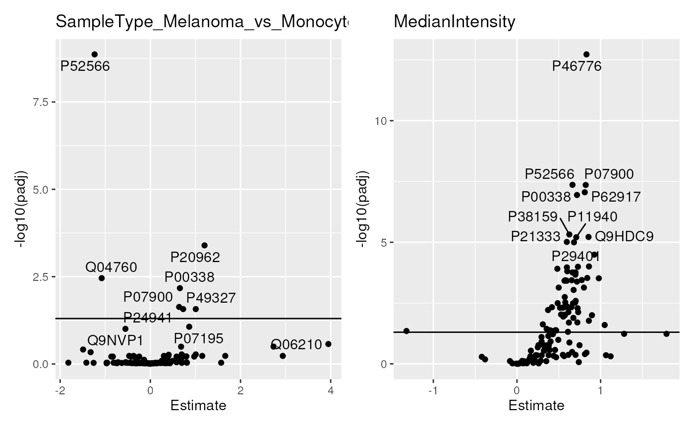
scpVolcanoPlot() takes the list of tables generated by scpDifferentialAnalysis() and returns a ggplot2 scatter plot. The plots show the adjusted p-values with respect to the estimate. A horizontal bar also highlights the significance threshold (defaults to 5%, fdrLine). The top (default 10) features with lowest p-values are labeled on the plot. You can control which features are labelled using the top, by and decreasing arguments. 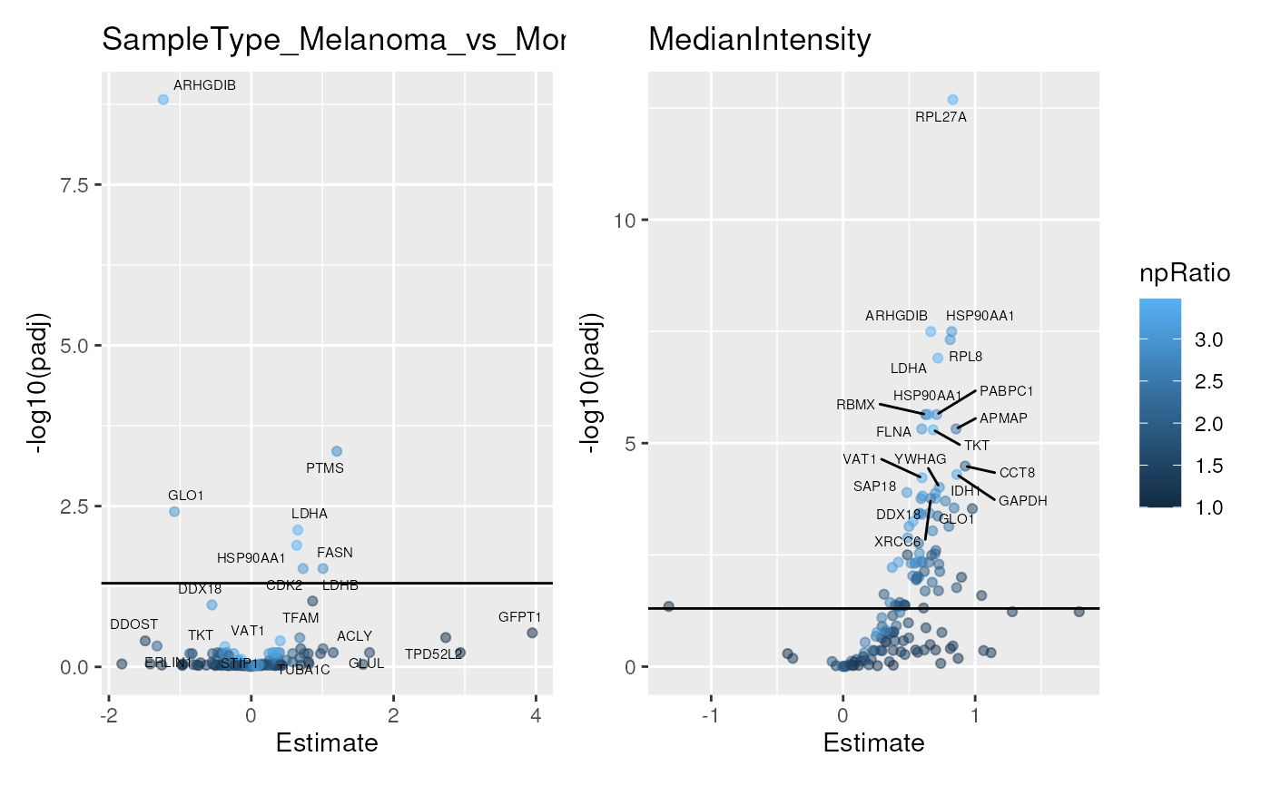Finally, you can change the point and label aesthetics thanks to the pointParams and the labelParams arguments, respectively.

See also

• ScpModel-Workflow to run a model on SCP data upstream of differential abundance analysis.

• scpAnnotateResults() to annotate analysis of variance results.

Author

Christophe Vanderaa, Laurent Gatto

Examples

library("patchwork")
library("ggplot2")
data("leduc_minimal")
## Add n/p ratio information in rowData
rowData(leduc_minimal)$npRatio <- 
    scpModelFilterNPRatio(leduc_minimal, filtered = FALSE)

####---- Run differential abundance analysis ----####

(res <- scpDifferentialAnalysis(
    leduc_minimal, coefficients =  "MedianIntensity", 
    contrasts = list(c("SampleType", "Melanoma", "Monocyte"))
))
#> Only 1 bin; IHW reduces to Benjamini Hochberg (uniform weights)
#> List of length 2
#> names(2): SampleType_Melanoma_vs_Monocyte MedianIntensity
## IHW return a message because of the example data set has only few
## peptides, real dataset should not have that problem.

####---- Annotate results ----####

## Add peptide annotations available from the rowData
res <- scpAnnotateResults(
    res, rowData(leduc_minimal), 
    by = "feature", by2 = "Sequence"
)

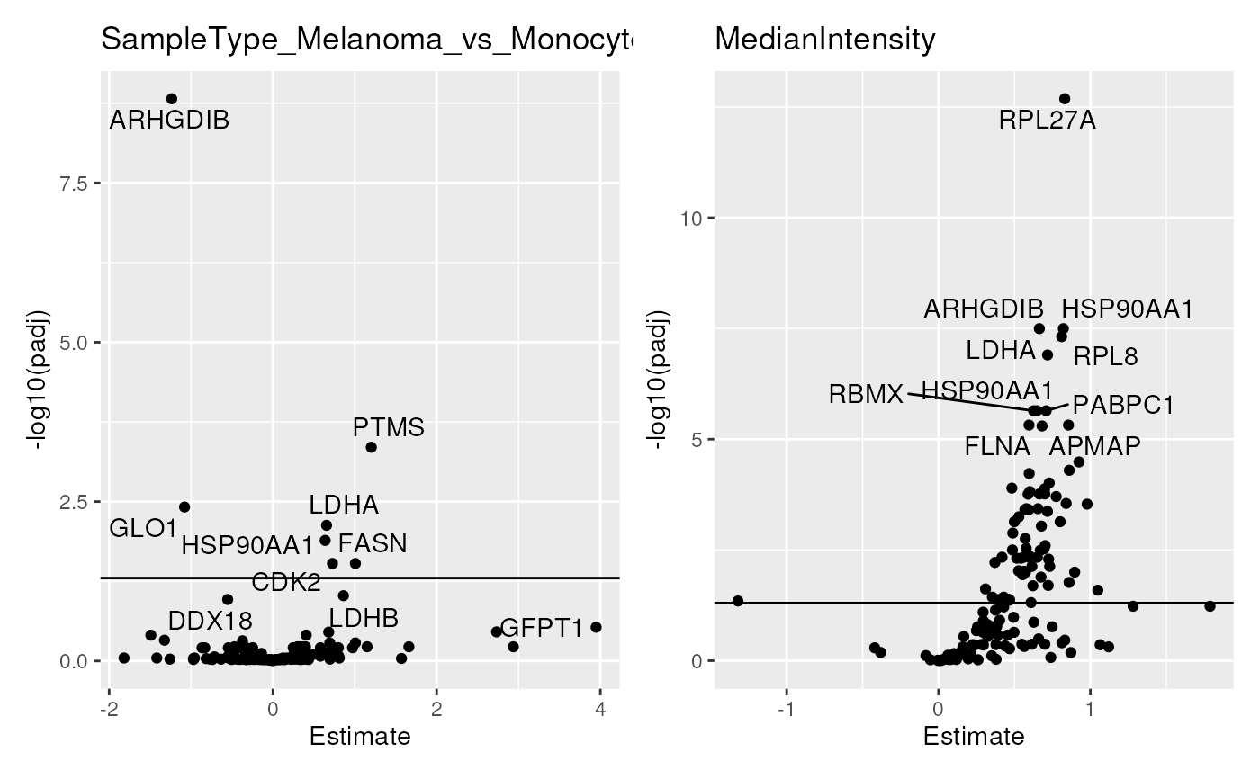
####---- Plot results ----####

scpVolcanoPlot(res, textBy = "gene") |>
    wrap_plots(guides = "collect")


## Modify point and label aesthetics
scpVolcanoPlot(
    res, textBy = "gene", top = 20,
    pointParams = list(aes(colour = npRatio), alpha = 0.5),
    labelParams = list(size = 2, max.overlaps = 20)) |>
    wrap_plots(guides = "collect")


####---- Aggregate results ----####

## Aggregate to protein-level results
byProteinDA <- scpDifferentialAggregate(
    res, fcol = "Leading.razor.protein.id"
)
scpVolcanoPlot(byProteinDA) |>
    wrap_plots(guides = "collect")