Replication of the cell cycle state study (Brunner et al. 2021)

Introduction

The study by Brunner et al. on the cell cycle is the first mass spectrometry-based single-cell proteomics (SCP) experiment that acquired hundreds of single cells using a label-free protocol (Brunner et al. (2022)). The data was acquired using a newly designed mass spectrometer that will later be released by Bruker as the timsTOF-SCP device. This instrument can be used for data dependent acquisition (DDA) or data independent acquisition (DIA). Single-cell samples were acquired using the latter and the DIA-NN software (Demichev et al. (2020)) was used to identify and quantify the MS data.

Let’s first load the replication package to make use of some helper functions. Those functions are only meant for this replication vignette and are not designed for general use.

library("SCP.replication")

`scp` and the plexDIA data analysis workflow

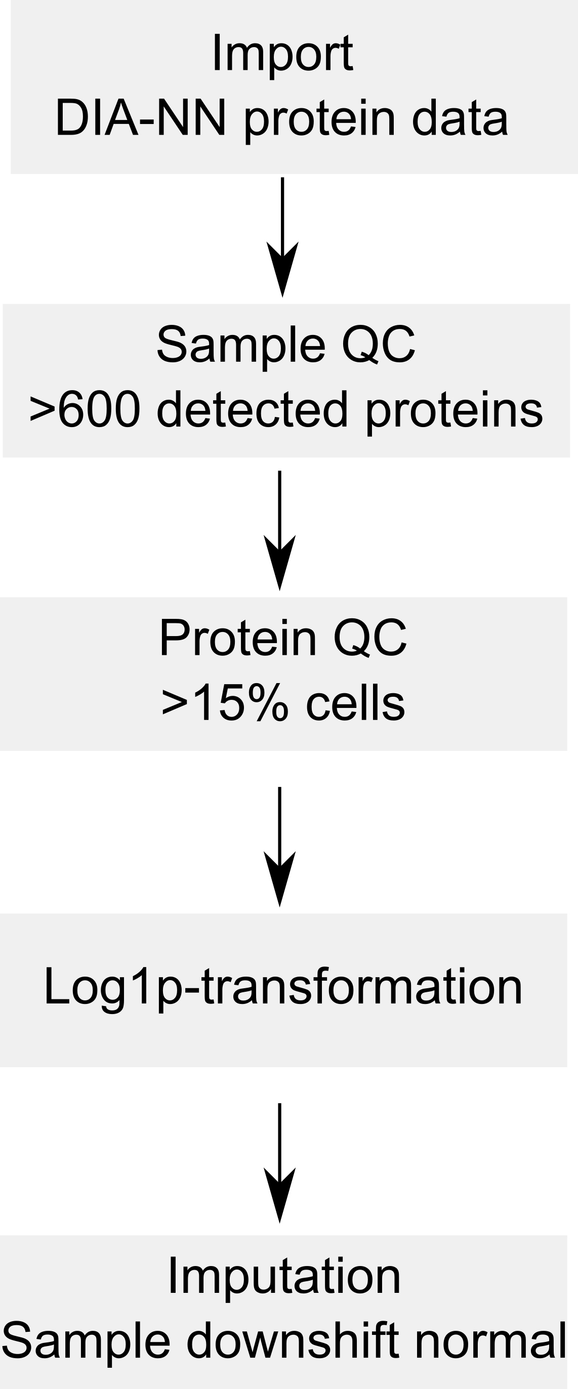
The code provided along with the article can be retrieved from this GitHub repository. It provides the python code used to reproduce the article’s analysis. The objective of this vignette is to replicate the analysis script using R code. We focus on standardized, easy-to-read, and well documented code. Therefore, our first contribution is to formalize the data processing into a conceptual flow chart.

Overview of the processing workflow by Derks et al.

This replication vignette relies on a data framework dedicated to SCP data analysis that combines two Bioconductor classes (Vanderaa and Gatto (2021)):

The SingleCellExperiment class provides an interface to many cutting edge methods for single-cell analysis
The QFeatures class facilitates manipulation and processing of MS-based quantitative data.

The scp vignette provides detailed information about the data structure. The scp package extends the functionality of QFeatures for single-cell application. scp offers a standardized implementation for single-cell processing methods.

The required packages for running this workflow are listed below.

## Core packages of this workflow
library("scp")
library("scpdata")
## External package for SingleCellExperiment objects
library("scater")
library("scuttle")
## Utility packages for data manipulation and visualization
library("tidyverse")
library("patchwork")

`scpdata` and the `brunner2022` dataset

We also implemented a data package called scpdata (Vanderaa and Gatto (2022)). It distributes published SCP datasets, such as the brunner2022 dataset. The datasets were downloaded from the data source provided in the publication and formatted to a QFeatures object so that it is compatible with our software. The underlying data storage is based on the ExperimentHub package that provides a cloud-based storage infrastructure.

The brunner2022 dataset is provided at different levels of processing:

The .d files that were generated by the mass-spectrometer. This data is not included in scpdata.
The DIA-NN main output report table that contains the results of the spectrum identification and quantification.
The DIA-NN protein group matrix: normalised quantities for protein groups, filtered at 1% FDR.
Other DIA-NN matrix: normalised quantities for precursors, gene groups or unique genes, filtered at 1% FDR. These files were not added to scpdata.

More information about the DIA-NN output tables can be found in the corresponding documentation.

The workflow starts with the protein group matrix and will replicate Figure 4 B, C and D from the original article. Note that the script did not mention which input file was used and we assumed from the methods section that the protein group matrix was used.

We formatted the brunner2022 dataset following the scp data framework. The formatted data can be retrieved from the scpdata package using the brunner2022() function. All datasets in scpdata are called after the first author and the date of publication. More information about the data and how it was processed can be find in ?brunner2022.

(brunner <- brunner2022())
## An instance of class QFeatures containing 435 assays:
##  [1] D:\Andreas_Brunner\Projects\SingleCellProteomics\202109_WorkHere\SingleCells\SingleShots_RawData\20201009_TIMS04_Evo07_AnBr_1Cell_HeLa_NB_01_S3-G2_1_3873.d: SingleCellExperiment with 3772 rows and 1 columns 
##  [2] D:\Andreas_Brunner\Projects\SingleCellProteomics\202109_WorkHere\SingleCells\SingleShots_RawData\20201009_TIMS04_Evo07_AnBr_1Cell_HeLa_NB_02_S3-G3_1_3874.d: SingleCellExperiment with 7759 rows and 1 columns 
##  [3] D:\Andreas_Brunner\Projects\SingleCellProteomics\202109_WorkHere\SingleCells\SingleShots_RawData\20201009_TIMS04_Evo07_AnBr_1Cell_HeLa_NB_03_S3-G4_1_3875.d: SingleCellExperiment with 4481 rows and 1 columns 
##  ...
##  [433] D:\Andreas_Brunner\Projects\SingleCellProteomics\202109_WorkHere\SingleCells\SingleShots_RawData\20201126_TIMS04_Evo07_SA_ADB_1cell_HeLa_UB_98_S2-C2_1_5109.d: SingleCellExperiment with 2569 rows and 1 columns 
##  [434] D:\Andreas_Brunner\Projects\SingleCellProteomics\202109_WorkHere\SingleCells\SingleShots_RawData\20201126_TIMS04_Evo07_SA_ADB_1cell_HeLa_UB_99_S2-C3_1_5110.d: SingleCellExperiment with 2327 rows and 1 columns 
##  [435] proteins: SingleCellExperiment with 2476 rows and 434 columns

The data are stored in a QFeatures object. In total, it contains 435 different SingleCellExperiment objects that we refer to as assays. Each assay contains expression data along with feature metadata. Each row in an assay represents a feature, in this case a precursor or a protein depending on the assay. Each column in an assay represents a sample. Each acquisition contains 1 cell, hence the precursor data contains 1 column per acquisition.

Using plot(), we can have a quick overview of the assays.

plot(brunner)
## Warning in plot.QFeatures(brunner): The QFeatures object contains many assays.
## You may want to consider creating an interactive plot (set 'interactive = TRUE')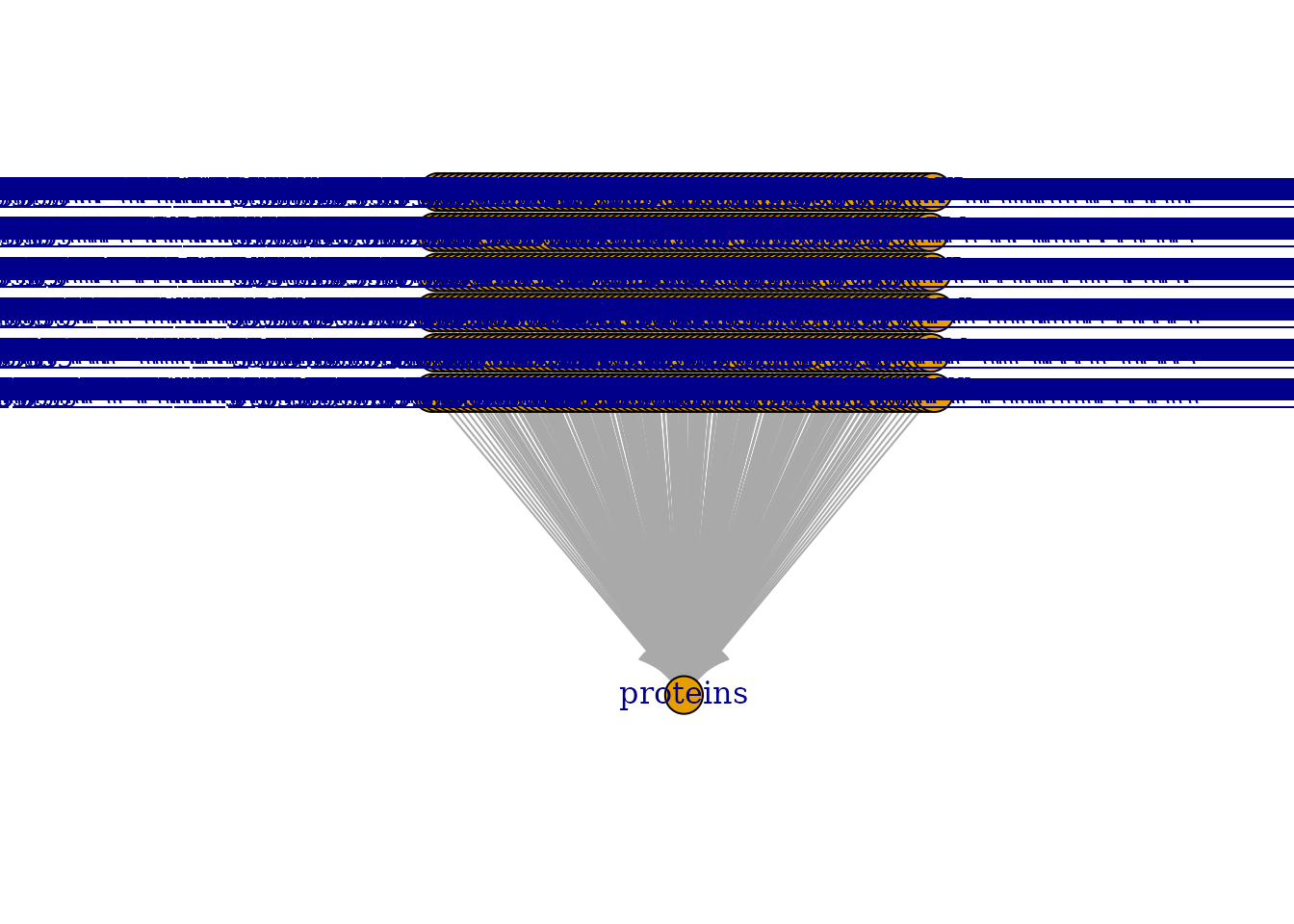

This figure is crowded, you can use plot(brunner, interactive = TRUE) to interactively explore this map. However, we can see that all precursor assays in the top of the figure are linked to the protein data.

Note that we inferred sample annotations from the file names. These are accessible from the colData.

colnames(colData(brunner))
##  [1] "File.Name"        "Run"              "Date"             "MsInstrument"    
##  [5] "Purification"     "User"             "SampleAnnotation" "SampleType"      
##  [9] "CellCycleStage"   "..undetermined.." "PlatePosition"    "CellNumber"      
## [13] "RunID"            "Label"

Filter cells

The authors first perform a sample quality control to make sure all cells have at least 600 quantified proteins. To perform this, we rely on perCellQCMetrics() from the scuttle package. To use this function we must first extract the assay we want to apply the function on, using double bracket subsetting ([[).

sce <- brunner[["proteins"]]

Next the function counts the number of features that are not zero, but missing data is encoded as NA. We therefore impote missing data with zero using impute() from the QFeatures package.

sce <- impute(sce, method = "zero")

We can now apply the QC function that will compute 3 metrics: the total abundance recorded per cell (sum and total, they are the same) and the number detected proteins per cell (detected).

cellqc <- perCellQCMetrics(sce, assay.type = 1)
colnames(cellqc)
## [1] "sum"      "detected" "total"

Next, we insert the computed metrics in the colData. This allows to use subsetByColData() and enable to subset single cells with 600 or more detected proteins.

colData(brunner)[, colnames(cellqc)] <- cellqc[rownames(colData(brunner)), ]
brunner <- subsetByColData(brunner, brunner$detected >= 600)

Filter proteins

The authors then filter for proteins that are detected in at least 15% of the cells. We apply the same procedure, but using perFeatureQCMetrics()

sce <- brunner[["proteins"]]
sce <- impute(sce, method = "zero")
protqc <- perFeatureQCMetrics(sce, assay.type = 1)
colnames(protqc)
## [1] "mean"     "detected"

perFeatureQCMetrics() computes the mean abundance for each protein (mean) and the detection rate across all cells (detected). Since this information is related to features, we must insert it in the rowData. This is a bit more complicated than for the colData since each assay has its own specific rowData. The QC metric we computed are related to the protein level and should only be included for the proteins assay. This can be done by providing a list. The name of the elements will indicate in which assay the rowData must be added. Columns of protqc are automatically added based on the protein names (see details in ?QFeatures-class for more details).

rowData(brunner) <- List(proteins = protqc)

Since the metrics are now in the rowData, we cannot use subsetByColData. Instead, we use filterFeatures() from the QFeatures package that will automactilly apply the filter on the rowData of each assay. Since detected is only available for proteins, we provide keep = TRUE to ignore the filter and hence keep the features for the other assays.

brunner <- filterFeatures(brunner, ~ detected > 0.15, 
                          keep = TRUE)

Performance assessment

In Figure 4 B and C of the original paper, the authors assessed the analytical performance of their technology for single-cell samples. The cells were analysed at different cell cycle stages thanks to thymidine and nocodazole block. We recode the annotation to match the corresponding cell cycle stage.

brunner$CellCycleStage <- recode(brunner$CellCycleStage,
                                 TB = "G1-S",
                                 NB = "G2-M",
                                 UB = "untreated")
table(brunner$CellCycleStage)
## 
##        G1      G1-S        G2      G2-M untreated 
##        87        41        52        45       203

The counts above are very close to those reported in the legend of Figure 4C. We next plot the number of quantified proteins per cell. This is already available from the colData. Using ggplot2, we replicate Figure 4B.

data.frame(colData(brunner)) %>% 
    rownames_to_column("id") %>% 
    ggplot() +
    aes(y = detected, 
        fill = CellCycleStage,
        color = CellCycleStage,
        x = id) +
    geom_bar(stat = "identity") +
    facet_grid(~ CellCycleStage, scales = "free_x", space = "free_x") +
    ylab("Quantified proteins") + xlab("") +
    theme(axis.text.x = element_blank(),
          axis.ticks = element_blank())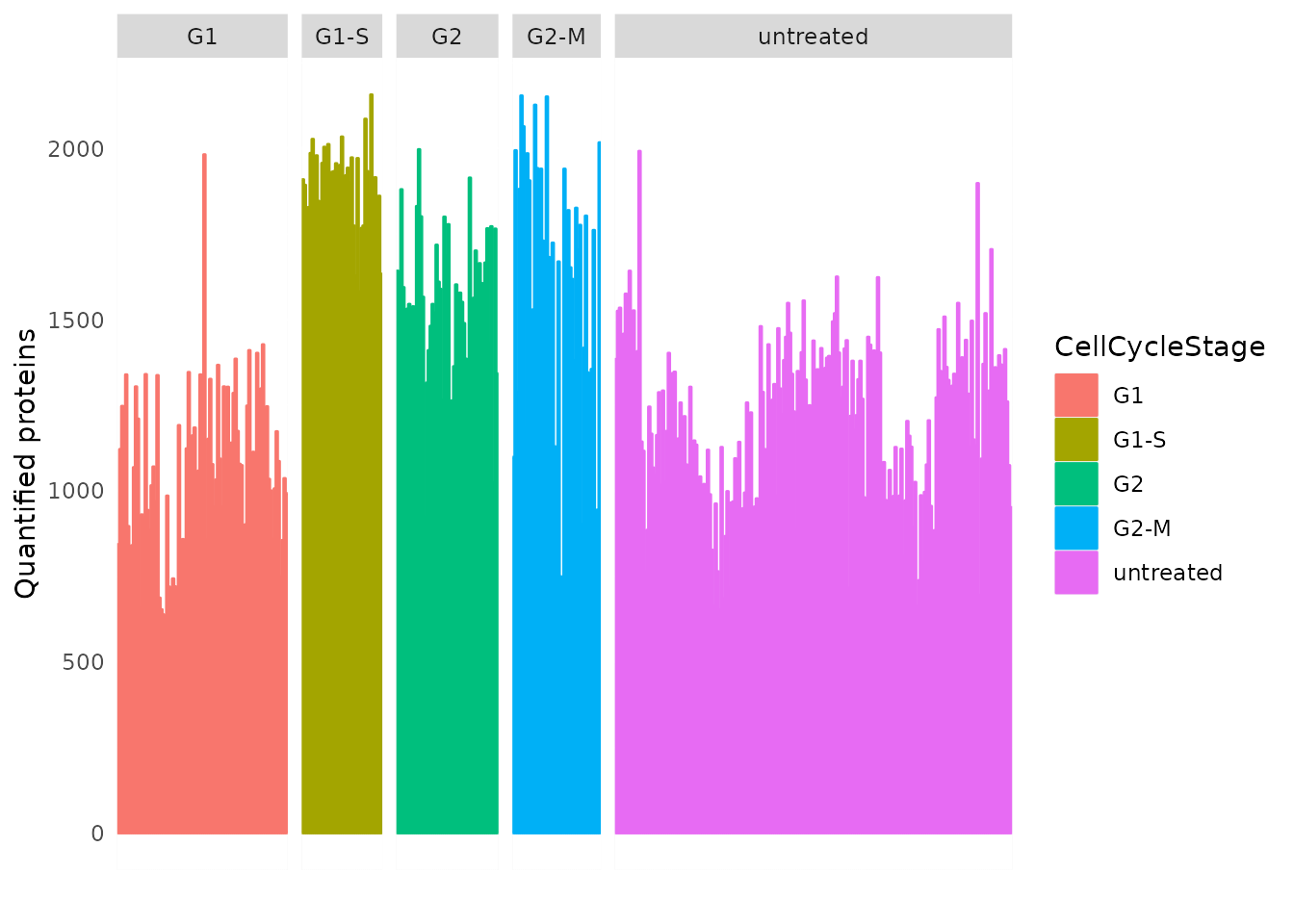

This plot is very similar to the original figure, except there here is the additional `“untreated”’ category.

We also plot the total signal per cell that replicated Figure 4C.

data.frame(colData(brunner)) %>% 
    ggplot() +
    aes(y = sum, 
        x = CellCycleStage,
        fill = CellCycleStage) +
    geom_boxplot() +
    theme_minimal()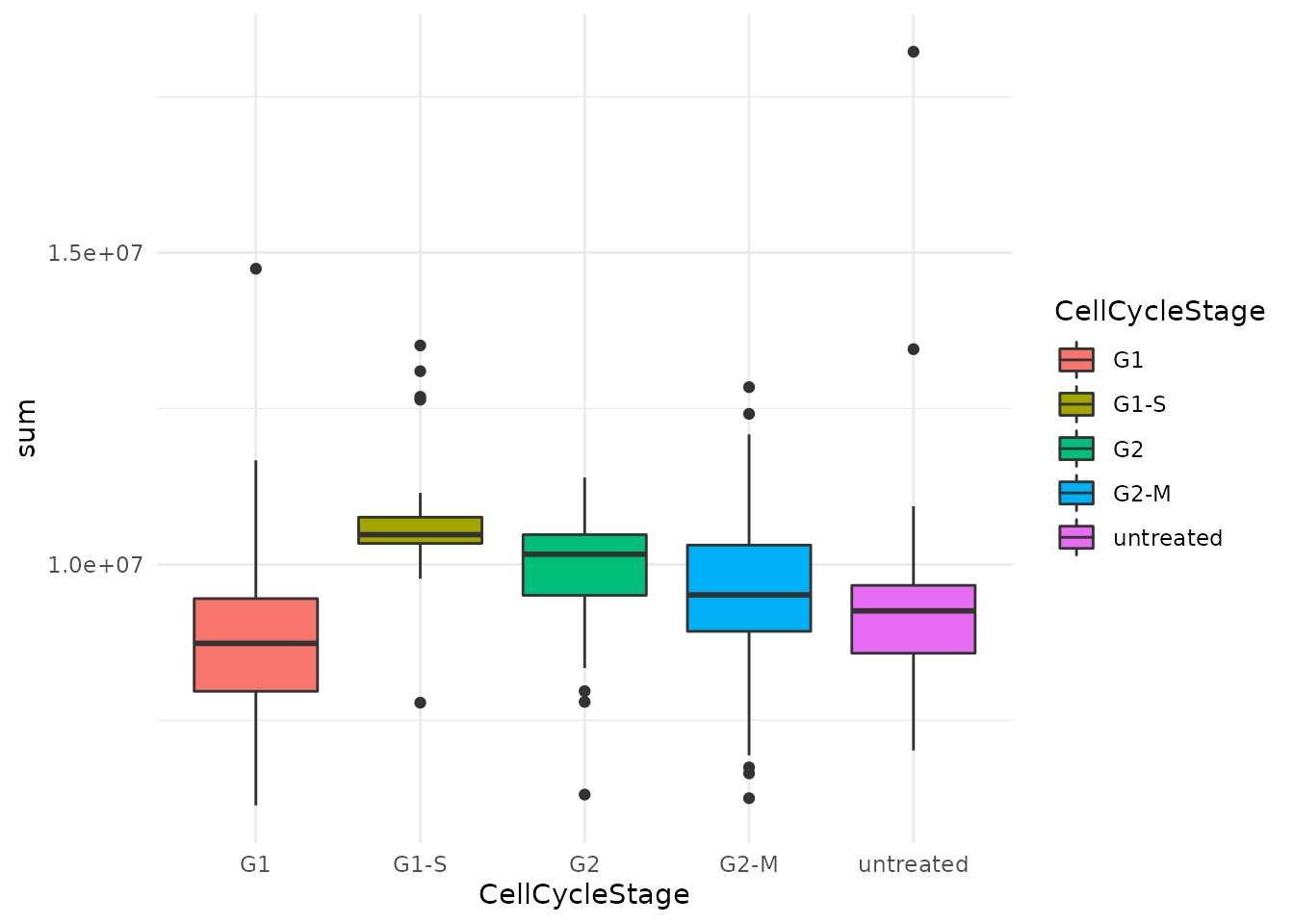

Log-Transformation

The protein data is then log2-transformed using logTransform(). This will add a new assay that we call proteins_log.

(brunner <- logTransform(brunner, i = "proteins", 
                        name = "proteins_log", 
                        base = exp(1), pc = 1))
## An instance of class QFeatures containing 436 assays:
##  [1] D:\Andreas_Brunner\Projects\SingleCellProteomics\202109_WorkHere\SingleCells\SingleShots_RawData\20201009_TIMS04_Evo07_AnBr_1Cell_HeLa_NB_01_S3-G2_1_3873.d: SingleCellExperiment with 3772 rows and 1 columns 
##  [2] D:\Andreas_Brunner\Projects\SingleCellProteomics\202109_WorkHere\SingleCells\SingleShots_RawData\20201009_TIMS04_Evo07_AnBr_1Cell_HeLa_NB_02_S3-G3_1_3874.d: SingleCellExperiment with 7759 rows and 1 columns 
##  [3] D:\Andreas_Brunner\Projects\SingleCellProteomics\202109_WorkHere\SingleCells\SingleShots_RawData\20201009_TIMS04_Evo07_AnBr_1Cell_HeLa_NB_03_S3-G4_1_3875.d: SingleCellExperiment with 4481 rows and 1 columns 
##  ...
##  [434] D:\Andreas_Brunner\Projects\SingleCellProteomics\202109_WorkHere\SingleCells\SingleShots_RawData\20201126_TIMS04_Evo07_SA_ADB_1cell_HeLa_UB_99_S2-C3_1_5110.d: SingleCellExperiment with 2327 rows and 1 columns 
##  [435] proteins: SingleCellExperiment with 2476 rows and 428 columns 
##  [436] proteins_log: SingleCellExperiment with 2476 rows and 428 columns

Imputation by downshifted norm

The final step is missing data imputation. As mentioned above, the QFeatures package has a function to perform imputation. The authors used imputation by sampling from a down-shifted normal distribution. Unfortunately, this method is not available, but we can provide it as a custom function.

imputeByDownShiftedNormal <- function(x, scale = 0.3, shift = 1.8) {
    m <- mean(x, na.rm = TRUE)
    std <- sd(x, na.rm = TRUE)
    nmis <- sum(is.na(x))
    repl <- rnorm(nmis, mean = m - shift * std, sd = scale * std)
    x[is.na(x)] <- repl
    x
}

We supply the custom function to impute()

brunner <- impute(brunner, i = "proteins_log", 
                  name = "proteins_dsnImpd",
                  FUN = imputeByDownShiftedNormal)

The last assay, proteins_dsnImpd, represents the final step of the data processing workflow.

PCA

We finally perform dimension reduction using PCA to replicate Figure 4D. This is performed by runPCA() and plotPCA() from the scater package. They work on SingleCEllExperiment objects and to include the sample annotation, we extract the last assay using getWithColData().

sce <- getWithColData(brunner, "proteins_dsnImpd")
## Warning: 'experiments' dropped; see 'metadata'
sce <- sce[, sce$CellCycleStage != "untreated"]
set.seed(1234)
sce <- runPCA(sce, ncomponents = 50,
              ntop = Inf,
              scale = TRUE,
              exprs_values = 1,
              name = "PCA")
plotPCA(sce, colour_by = "CellCycleStage") +
    scale_colour_manual(values = c("darkseagreen", "cornflowerblue", 
                                   "grey", "darkorange2"))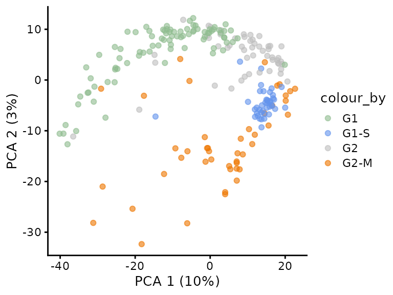

This plot shows similar trends to the original figure although the percent variability explained is lower in our replication (PC1: 10 vs 14% and PC2: 3 vs 4 %).

An important aspect of the data analysis that the authors overlooked is the assessment of batch effect. We extracted the (presumably) date of acquisition from the file names and plot these on the PCA.

plotPCA(sce, colour_by = "Date") +
    scale_colour_manual(values = c("gold", "gold3", "orange2", "orange4"))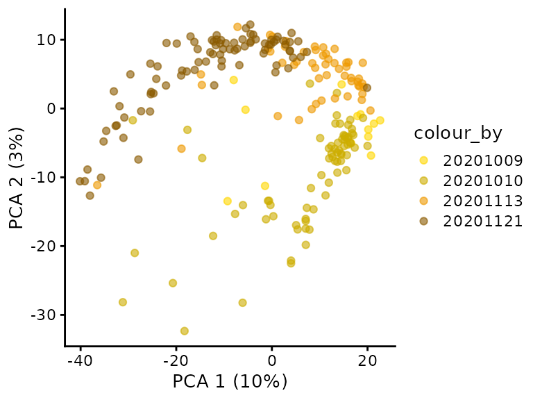

Surprisingly, we observe the different cell cycle stages where acquired in distinct batches. For instance, all G1 cells where acquired on November 21, 2020 and all G2 cells where acquired on November 13, 2020. This is an issue because batch effects can dramatically influence quantifications in proteomics experiments, especially SCP (Vanderaa and Gatto (2021)). This experimental design does not allow for batch correction and hence we cannot distinguish the proportion of variance that is explained by technical and biological factors…

In the article, the authors argue:

In addition to these drug-perturbed cells, we measured more than 200 untreated ones from two independent cell culture batches. The proteomes of these asynchronous cells distributed well across the cell cycle states, while different passage batches were enriched in the G1 and G2 phase

They refer to supplementary Figure EV2E. Let’s replicate this figure:

sce <- getWithColData(brunner, "proteins_dsnImpd")
## Warning: 'experiments' dropped; see 'metadata'
set.seed(1234)
sce <- runPCA(sce, ncomponents = 50,
              ntop = Inf,
              scale = TRUE,
              exprs_values = 1,
              name = "PCA")
plotPCA(sce, colour_by = "CellCycleStage") +
    scale_colour_manual(values = c("darkseagreen", "cornflowerblue", 
                                   "grey", "darkorange2", "firebrick"))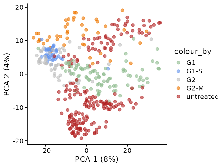

Indeed, we also find that some untreated cells are close to G1 cells in PCA space and other are closer to the G2-M phase. But let’s look at the batch effect.

plotPCA(sce, colour_by = "Date") +
    scale_colour_manual(values = c("gold", "gold3", "orange2", "orange4","red4"))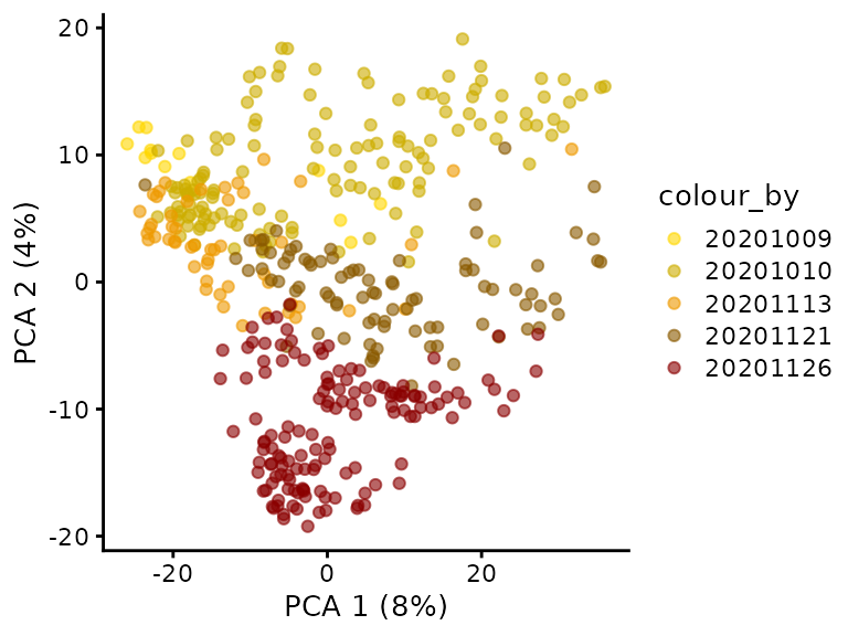

The PCA better explains the acquisition date than the cells cycle stage, refuting the argument stated above. A better design would have been to randomize the cell cycle stages across several acquisition runs. Obviously, effect of cell culture batch or FACS sorting may be responsible as well and are practically inevitably. Spreading sample preparation over several culture and FACS sorting batches would have allowed to disentangle the biological and technical variability.

Conclusion

This vignette present a standardized R solution to replicate the python analysis by Brunner et al. (2022). We successfully reproduced their main results for the SCP cell cycle experiment. By re-analyzing the data, we discovered an important flaw in the experimental design. Technical and biological factors cannot be distinguished hindering batch correction, leading to potentially biased outcome.

Reproduce this vignette

You can reproduce this vignette using Docker:

docker pull cvanderaa/scp_replication_docker:v1
docker run \
    -e PASSWORD=bioc \
    -p 8787:8787 \
    cvanderaa/scp_replication_docker:v1

Open your browser and go to http://localhost:8787. The USER is rstudio and the password is bioc. You can find the vignette in the vignettes folder.

See the website home page for more information.

Requirements

Hardware and software

The system details of the machine that built the vignette are:

## Machine: Linux (5.15.0-48-generic)
## R version: R.4.2.1 (svn: 82513)
## RAM: 16.5 GB
## CPU: 16 core(s) - 11th Gen Intel(R) Core(TM) i7-11800H @ 2.30GHz

Timing

The total time required to compile this vignette is:

## 7.945226 mins

Memory

The final leduc object size is:

## [1] "2.3 Gb"

Session info

sessionInfo()
## R version 4.2.1 (2022-06-23)
## Platform: x86_64-pc-linux-gnu (64-bit)
## Running under: Ubuntu 20.04.4 LTS
## 
## Matrix products: default
## BLAS:   /usr/lib/x86_64-linux-gnu/blas/libblas.so.3.9.0
## LAPACK: /usr/lib/x86_64-linux-gnu/lapack/liblapack.so.3.9.0
## 
## locale:
##  [1] LC_CTYPE=en_US.UTF-8       LC_NUMERIC=C              
##  [3] LC_TIME=en_US.UTF-8        LC_COLLATE=en_US.UTF-8    
##  [5] LC_MONETARY=en_US.UTF-8    LC_MESSAGES=en_US.UTF-8   
##  [7] LC_PAPER=en_US.UTF-8       LC_NAME=C                 
##  [9] LC_ADDRESS=C               LC_TELEPHONE=C            
## [11] LC_MEASUREMENT=en_US.UTF-8 LC_IDENTIFICATION=C       
## 
## attached base packages:
## [1] stats4    stats     graphics  grDevices utils     datasets  methods  
## [8] base     
## 
## other attached packages:
##  [1] benchmarkme_1.0.8           patchwork_1.1.2            
##  [3] forcats_0.5.2               stringr_1.4.1              
##  [5] dplyr_1.0.10                purrr_0.3.4                
##  [7] readr_2.1.3                 tidyr_1.2.1                
##  [9] tibble_3.1.8                tidyverse_1.3.2            
## [11] scater_1.25.7               ggplot2_3.3.6              
## [13] scuttle_1.7.4               SCP.replication_0.2.1      
## [15] SingleCellExperiment_1.19.1 scpdata_1.5.4              
## [17] ExperimentHub_2.5.0         AnnotationHub_3.5.2        
## [19] BiocFileCache_2.5.0         dbplyr_2.2.1               
## [21] scp_1.7.4                   QFeatures_1.7.3            
## [23] MultiAssayExperiment_1.23.9 SummarizedExperiment_1.27.3
## [25] Biobase_2.57.1              GenomicRanges_1.49.1       
## [27] GenomeInfoDb_1.33.7         IRanges_2.31.2             
## [29] S4Vectors_0.35.4            BiocGenerics_0.43.4        
## [31] MatrixGenerics_1.9.1        matrixStats_0.62.0         
## [33] BiocStyle_2.25.0           
## 
## loaded via a namespace (and not attached):
##   [1] utf8_1.2.2                    reticulate_1.26              
##   [3] tidyselect_1.1.2              RSQLite_2.2.17               
##   [5] AnnotationDbi_1.59.1          grid_4.2.1                   
##   [7] BiocParallel_1.31.12          munsell_0.5.0                
##   [9] ScaledMatrix_1.5.1            codetools_0.2-18             
##  [11] ragg_1.2.3                    withr_2.5.0                  
##  [13] colorspace_2.0-3              filelock_1.0.2               
##  [15] highr_0.9                     knitr_1.40                   
##  [17] labeling_0.4.2                GenomeInfoDbData_1.2.9       
##  [19] bit64_4.0.5                   farver_2.1.1                 
##  [21] rprojroot_2.0.3               vctrs_0.4.2                  
##  [23] generics_0.1.3                xfun_0.33                    
##  [25] doParallel_1.0.17             R6_2.5.1                     
##  [27] ggbeeswarm_0.6.0              clue_0.3-61                  
##  [29] rsvd_1.0.5                    locfit_1.5-9.6               
##  [31] MsCoreUtils_1.9.1             AnnotationFilter_1.21.0      
##  [33] bitops_1.0-7                  cachem_1.0.6                 
##  [35] DelayedArray_0.23.2           assertthat_0.2.1             
##  [37] promises_1.2.0.1              scales_1.2.1                 
##  [39] googlesheets4_1.0.1           beeswarm_0.4.0               
##  [41] gtable_0.3.1                  beachmat_2.13.4              
##  [43] OrgMassSpecR_0.5-3            benchmarkmeData_1.0.4        
##  [45] sva_3.45.0                    rlang_1.0.6                  
##  [47] genefilter_1.79.0             systemfonts_1.0.4            
##  [49] splines_4.2.1                 lazyeval_0.2.2               
##  [51] gargle_1.2.1                  broom_1.0.1                  
##  [53] BiocManager_1.30.18           yaml_2.3.5                   
##  [55] modelr_0.1.9                  backports_1.4.1              
##  [57] httpuv_1.6.6                  tools_4.2.1                  
##  [59] bookdown_0.29                 ellipsis_0.3.2               
##  [61] jquerylib_0.1.4               Rcpp_1.0.9                   
##  [63] sparseMatrixStats_1.9.0       zlibbioc_1.43.0              
##  [65] RCurl_1.98-1.9                viridis_0.6.2                
##  [67] cowplot_1.1.1                 haven_2.5.1                  
##  [69] ggrepel_0.9.1                 cluster_2.1.4                
##  [71] fs_1.5.2                      magrittr_2.0.3               
##  [73] reprex_2.0.2                  googledrive_2.0.0            
##  [75] ProtGenerics_1.29.0           hms_1.1.2                    
##  [77] mime_0.12                     evaluate_0.16                
##  [79] xtable_1.8-4                  XML_3.99-0.11                
##  [81] readxl_1.4.1                  gridExtra_2.3                
##  [83] compiler_4.2.1                crayon_1.5.2                 
##  [85] htmltools_0.5.3               mgcv_1.8-40                  
##  [87] later_1.3.0                   tzdb_0.3.0                   
##  [89] lubridate_1.8.0               DBI_1.1.3                    
##  [91] MASS_7.3-58.1                 rappdirs_0.3.3               
##  [93] Matrix_1.5-1                  cli_3.4.1                    
##  [95] parallel_4.2.1                igraph_1.3.5                 
##  [97] pkgconfig_2.0.3               pkgdown_2.0.6                
##  [99] foreach_1.5.2                 xml2_1.3.3                   
## [101] annotate_1.75.0               vipor_0.4.5                  
## [103] bslib_0.4.0                   XVector_0.37.1               
## [105] rvest_1.0.3                   digest_0.6.29                
## [107] Biostrings_2.65.6             rmarkdown_2.16               
## [109] cellranger_1.1.0              edgeR_3.39.6                 
## [111] DelayedMatrixStats_1.19.1     curl_4.3.2                   
## [113] shiny_1.7.2                   lifecycle_1.0.2              
## [115] nlme_3.1-159                  jsonlite_1.8.2               
## [117] BiocNeighbors_1.15.1          desc_1.4.2                   
## [119] viridisLite_0.4.1             limma_3.53.10                
## [121] fansi_1.0.3                   pillar_1.8.1                 
## [123] lattice_0.20-45               KEGGREST_1.37.3              
## [125] fastmap_1.1.0                 httr_1.4.4                   
## [127] survival_3.4-0                interactiveDisplayBase_1.35.0
## [129] glue_1.6.2                    iterators_1.0.14             
## [131] png_0.1-7                     BiocVersion_3.16.0           
## [133] bit_4.0.4                     stringi_1.7.8                
## [135] sass_0.4.2                    BiocBaseUtils_0.99.12        
## [137] blob_1.2.3                    textshaping_0.3.6            
## [139] BiocSingular_1.13.1           memoise_2.0.1                
## [141] irlba_2.3.5.1

Licence

This vignette is distributed under a CC BY-SA licence licence.

References

Brunner, Andreas-David, Marvin Thielert, Catherine Vasilopoulou, Constantin Ammar, Fabian Coscia, Andreas Mund, Ole B Hoerning, et al. 2022. “Ultra-High Sensitivity Mass Spectrometry Quantifies Single-Cell Proteome Changes Upon Perturbation.” Mol. Syst. Biol. 18 (3): e10798.

Demichev, Vadim, Christoph B Messner, Spyros I Vernardis, Kathryn S Lilley, and Markus Ralser. 2020. “DIA-NN: Neural Networks and Interference Correction Enable Deep Proteome Coverage in High Throughput.” Nat. Methods 17 (1): 41–44.

Vanderaa, Christophe, and Laurent Gatto. 2021. “Replication of Single-Cell Proteomics Data Reveals Important Computational Challenges.” Expert Rev. Proteomics, October.

———. 2022. “The Current State of Single-Cell Proteomics Data Analysis,” October. https://arxiv.org/abs/2210.01020.

Christophe Vanderaa, Computational Biology, UCLouvain

Laurent Gatto, Computational Biology, UCLouvain

5 October 2022

Introduction

`scp` and the plexDIA data analysis workflow

`scpdata` and the `brunner2022` dataset

Filter cells

Filter proteins

Performance assessment

Log-Transformation

Imputation by downshifted norm

PCA

Conclusion

Reproduce this vignette

Requirements

Hardware and software

Timing

Memory

Session info

Licence

References

Replication of the cell cycle state study (Brunner et al. 2021)

Christophe Vanderaa, Computational Biology, UCLouvain

Laurent Gatto, Computational Biology, UCLouvain

5 October 2022

Introduction

scp and the plexDIA data analysis workflow

scpdata and the brunner2022 dataset

Filter cells

Filter proteins

Performance assessment

Log-Transformation

Imputation by downshifted norm

PCA

Conclusion

Reproduce this vignette

Requirements

Hardware and software

Timing

Memory

Session info

Licence

References

`scp` and the plexDIA data analysis workflow

`scpdata` and the `brunner2022` dataset