Replication of the plexDIA analysis (Derks et al. 2022)
Christophe Vanderaa1, Computational Biology, UCLouvain
Laurent Gatto, Computational Biology, UCLouvain
5 October 2022
derks2022.RmdIntroduction
plexDIA (Derks et al. (2022)) enables the profiling of the proteome of single cells using a multiplexed DIA data acquisition strategy. The pipeline includes the nPOP sample processing protocole (Leduc, Gray Huffman, and Slavov (2022)), with mTRAQ labeling of the samples. The authors used the DIA-NN software (Demichev et al. (2020)) to identify and quantify the MS data.
Let’s first load the replication package to make use of some helper functions. Those functions are only meant for this replication vignette and are not designed for general use.
library("SCP.replication")
scp and the plexDIA data analysis workflow
The code provided along with the article can be retrieved from this GitHub repository. The objective of this vignette is to replicate the analysis script while providing standardized, easy-to-read, and well documented code. Therefore, our first contribution is to formalize the data processing into a conceptual flow chart.
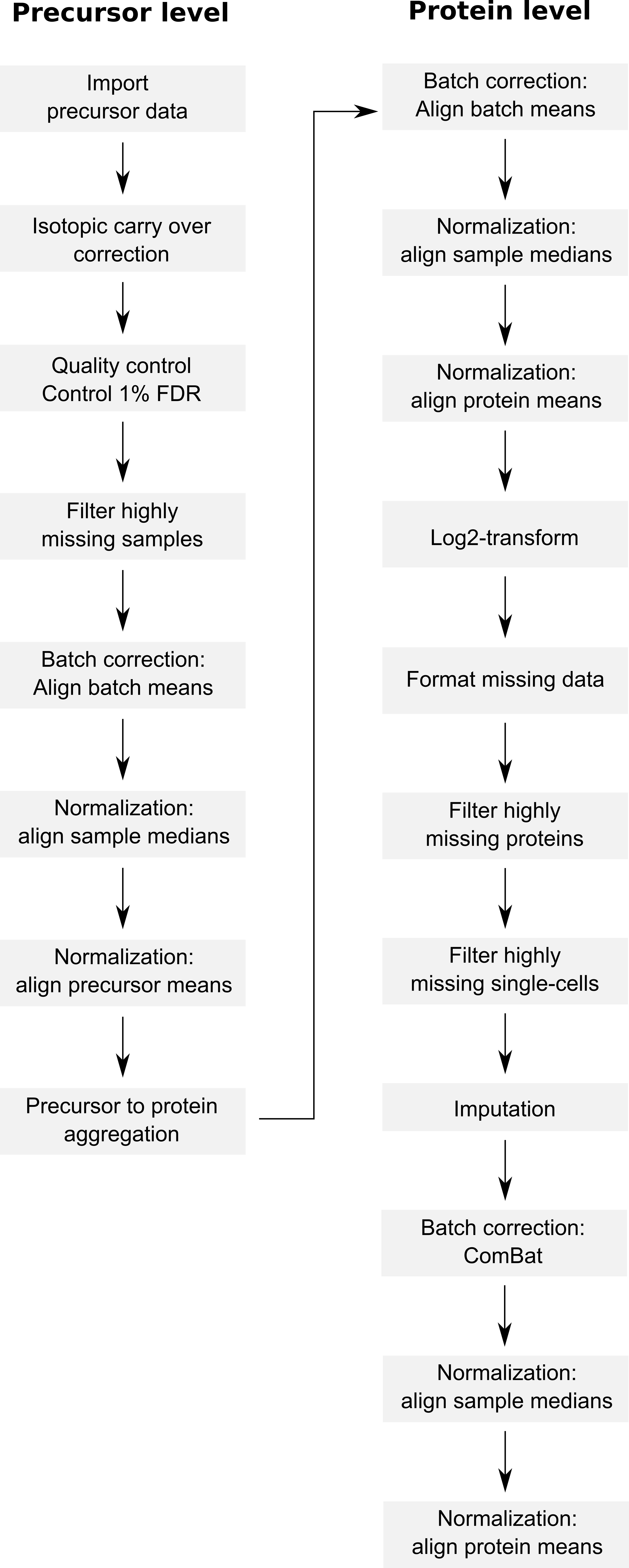
Overview of the processing workflow by Derks et al.
This replication vignette relies on a data framework dedicated to SCP data analysis that combines two Bioconductor classes (Vanderaa and Gatto (2021)):
- The
SingleCellExperimentclass provides an interface to many cutting edge methods for single-cell analysis - The
QFeaturesclass facilitates manipulation and processing of MS-based quantitative data.
The scp
vignette provides detailed information about the data structure. The
scp package extends the functionality of
QFeatures for single-cell application. scp
offers a standardized implementation for single-cell processing
methods.
The required packages for running this workflow are listed below.
## Core packages of this workflow
library("scp")
library("scpdata")
library("sva")

## Utility packages for data manipulation and visualization
library("tidyverse")
library("ggbeeswarm")
library("ggrepel")
library("patchwork")
library("ggpointdensity")
scpdata and the leduc2022 dataset
We also implemented a data package called scpdata (Vanderaa and Gatto (2022)). It distributes
published SCP datasets, such as the derks2022 dataset. The
datasets were downloaded from the data source provided in the
publication and formatted to a QFeatures object so that it
is compatible with our software. The underlying data storage is based on
the ExperimentHub package that provides a cloud-based
storage infrastructure.
The derks2022 dataset is provided at different levels of
processing:
- The .raw and .d files that were generated by the
mass-spectrometers. This data is not included in
scpdata. - The DIA-NN main output report table that contains the results of the spectrum identification and quantification.
- The DIA-NN MS1 extracted signal table, if a precursor was identified in at least one of the mTRAQ channels in the main report, signal (if any) will be extracted from the other channels regardless of whether there is sufficient evidence in those channels at 1% FDR.
- A processed protein data table is provided as the final output of the data processing. This workflow will try to replicate this table.
The workflow starts with precursor tables and will generate the processed protein data. The authors provided the DIA-NN output tables and the sample annotation table through a Google Drive repo. Protein data are shared a TXT files. We highly value the effort the authors have made to publicly share all the data generated in their project, from raw files to final expression tables (see the Slavov Lab website).
We formatted the derks2022 dataset following our data
framework. The formatted data can be retrieved from the
scpdata package using the derks2022()
function. All datasets in scpdata are called after the
first author and the date of publication.
The derks2022 data combines 3 main datasets: the
100-cell equivalent samples acquired with a Q-Exactive instrument, the
single-cell samples acquired with a Q-Exactive instrument (we call this
dataset qe), and the the single-cell samples acquired with
a timsTOF-SCP instrument (we call this dataset tims). Each
dataset contains the DIA-NN main report data split over each run and the
combined MS1 extracted data (see above for more details). The data also
contains the protein data for all samples as processed by the
authors.
(derks <- derks2022())
## An instance of class QFeatures containing 66 assays:
##  [1] F..JD.plexDIA.nPOP.wJD1194.raw: SingleCellExperiment with 19618 rows and 3 columns
##  [2] F..JD.plexDIA.nPOP.wJD1195.raw: SingleCellExperiment with 19587 rows and 3 columns
##  [3] F..JD.plexDIA.nPOP.wJD1196.raw: SingleCellExperiment with 19176 rows and 3 columns
##  ...
##  [64] F..JD.plexDIA.nPOP.wJD1193.raw: SingleCellExperiment with 2643 rows and 3 columns
##  [65] qe_prec_extracted: SingleCellExperiment with 8590 rows and 144 columns
##  [66] proteins: SingleCellExperiment with 1475 rows and 164 columns
The datasets are stored in a QFeatures object. In total,
it contains 66 different SingleCellExperiment objects that
we refer to as assays. Each assay contains expression
data along with feature metadata. Each row in an assay represents a
feature, in this case a precursor or a protein
depending on the assay. Each column in an assay represents a
sample. During sample preparation, 3 samples are pooled
using mTRAQ labeling, hence some assays contain 3 columns corresponding
to each measured channel.
Using plot(), we can have a quick overview of the
assays.
plot(derks)
## Warning in plot.QFeatures(derks): The QFeatures object contains many assays. You
## may want to consider creating an interactive plot (set 'interactive = TRUE')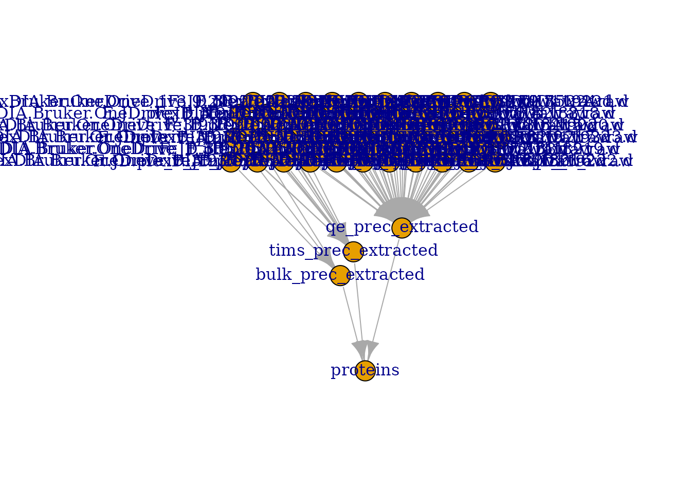
This figure is crowded, you can use
plot(derks, interactive = TRUE) to interactively explore
this map. However, we can see that the different runs in the top of the
figure converge to 3 assays that contain the extracted MS1 precursor
signal for the three datasets: bulk, tims and
qe. Finally, the protein table contains data derived from
all three datasets.
The objective of this vignette is to replicate the combined protein data table from the precursor assays following the same data processing workflow as the original study by Derks et al. but using standardized functionality.
We extract the proteins assay and keep it for later
benchmarking. getWithColData() extract an assay of interest
along with the associated sample annotations. We then remove the assay
from the S object for the remainder of the processing. We
apply this using removeAssays.
proteins_derks <- getWithColData(derks, "proteins")
## Warning: 'experiments' dropped; see 'metadata'
## Warning: Ignoring redundant column names in 'colData(x)':
derks <- removeAssay(derks, "proteins")
## Warning: 'experiments' dropped; see 'metadata'
Remove unwanted samples
Before starting the data processing, we remove the samples that are
not considered by the authors to generate the protein data. The
timsTOF-SCP dataset was acquired with a few bulk samples diluted to
single-cell equivalent. These samples are ending with
"_t_DB". The Q-Exactive dataset contains single-cells, but
also a dozen negative controls (encoded as "Neg").
table(derks$Celltype, derks$dataset)
##
##                 bulk Q-Exactive timsTOFSCP
##   Melanoma         0         45          0
##   Melanoma_DB      3          0          0
##   Melanoma_t       0          0         10
##   Melanoma_t_DB    0          0          1
##   Neg              0         12          0
##   PDAC             0         45          0
##   PDAC_DB          3          0          0
##   PDAC_t           0          0         10
##   PDAC_t_DB        0          0          1
##   U-937            0         42          0
##   U-937_DB         3          0          0
##   U-937_t          0          0         10
##   U-937_t_DB       0          0          1
We remove those unwanted samples by accessing the information from
the colData using subsetByColData().
derks <- subsetByColData(derks, !grepl("Neg|_t_DB", derks$Celltype))Isotopic carry over correction
The first data processing step is to correct for isotopic carry over
from one mTRAQ channel to another. This is performed using
correctIsotopicCarryover(). The function takes an assay and
returns the same assay with corrected quantifications. Since there are 3
datasets, we will loop over the 3 assays containing the extracted MS1
signal. These corrected assays are added to the QFeatures
object using addAssay() and the links between the
precursors are added using
for (i in c("bulk", "qe", "tims")) {
    inputAssay <- paste0(i ,"_prec_extracted")
    outputAssay <- paste0(i ,"_prec_corrected")
    x <- correctIsotopicCarryover(derks[[inputAssay]])
    derks <- addAssay(derks, x, name = outputAssay)
    derks <- addAssayLinkOneToOne(derks, from = inputAssay,
                                  to = outputAssay)
    cat("Finished correction for the", i, "dataset\n")
}
## Finished correction for the bulk dataset
## Finished correction for the qe dataset
## Finished correction for the tims dataset
Precursor FDR control
Precursors are then filtered to control for protein FDR. To perform
this, we will again loop over the 3 datasets as the set of protein that
comply to the FDR threshold is dataset-dependent. We retrieve the assays
that link to extracted signal assay as these contain the FDR threshold.
Once identified, we combine all the available rowData in a
single table using rbindRowData(). This table is then
filtered to retrieve the proteins with low FDR and we subset the
corrected signal assay to contain only precursors that map those
proteins. Finally, we restore any lost link between the precursors of
corrected assay with its parent assay using
addAssayLink().
for (i in c("bulk", "qe", "tims")) {
    ## Find the assays that contain the FDR (q-value) information
    repAssays <- assayLink(derks, paste0(i ,"_prec_extracted"))@from
    ## Combine all rowData in a single table
    rd <- rbindRowData(derks, repAssays)
    ## Perform filtering
    PGs_0.01FDR <- unique(rd$Protein.Group[rd$Lib.PG.Q.Value < 0.01])
    ## Apply the filter to the corrected signal assay
    x <- derks[[paste0(i ,"_prec_corrected")]]
    ind <- rowData(x)$Protein.Group %in% PGs_0.01FDR
    derks[[paste0(i ,"_prec_corrected")]] <- x[ind, ]
    ## AssayLinks are lost when removing proteins, we recreate them
    derks <- addAssayLink(derks, from = paste0(i ,"_prec_extracted"),
                          to = paste0(i ,"_prec_corrected"),
                          varFrom = "Precursor.Id",
                          varTo = "Precursor.Id")
    cat("Finished FDR control for the", i, "dataset\n")
}
## Finished FDR control for the bulk dataset
## Warning in replaceAssay(x = x, y = value, i = i): Links between assays were
## lost/removed during replacement. See '?addAssayLink' to restore them manually.
## Finished FDR control for the qe dataset
## Finished FDR control for the tims dataset
discussion you find this chuk too complicated? Let’s discuss this by opening an issue here.
Combine the datasets
Up to now, we kept the data belonging to each MS run in separate
assays. We now combine all batches into a single assay. This can easily
be done using the joinAssays() function from the
QFeatures package.
Consensus mapping of precursors to proteins
We need to account for a limitation when combining the data.
joinAssays() will only keep the metadata variables that
have the same value between matching rows. However, some precursors map
to one protein group in one run and to another protein group in another
run. Hence, the protein group is not constant for all precursors and is
removed during joining. It is important we keep the protein group
information in the rowData since we will later need it to
aggregate precursors to proteins. To avoid this issue, we replace the
problematic precursor to protein group mappings through a majority
vote.
## Generate a list of DataFrames with the information to modify
precAssays <- grep("corrected$", names(derks), value = TRUE)
ppMap <- rbindRowData(derks, i = precAssays) %>%
    data.frame %>%
    group_by(Precursor.Id) %>%
    ## The majority vote happens here
    mutate(Protein.Group =
               names(sort(table(Protein.Group),
                          decreasing = TRUE))[1]) %>%
    select(Precursor.Id, Protein.Group) %>%
    filter(!duplicated(Precursor.Id, Protein.Group))
consensus <- lapply(precAssays, function(i) {
    ind <- match(rowData(derks[[i]])$Precursor.Id,
                 ppMap$Precursor.Id)
    DataFrame(Protein.Group = ppMap$Protein.Group[ind])
})
## Name the list
names(consensus) <- precAssays
## Modify the rowData
rowData(derks) <- consensus
We now join the three datasets in a single assay. This is performed
using joinAssays().
(derks <- joinAssays(derks, i = grep("corrected$", names(derks)),
                     name = "prec_corrected"))
## An instance of class QFeatures containing 69 assays:
##  [1] F..JD.plexDIA.nPOP.wJD1194.raw: SingleCellExperiment with 19618 rows and 3 columns
##  [2] F..JD.plexDIA.nPOP.wJD1195.raw: SingleCellExperiment with 19587 rows and 3 columns
##  [3] F..JD.plexDIA.nPOP.wJD1196.raw: SingleCellExperiment with 19176 rows and 3 columns
##  ...
##  [67] qe_prec_corrected: SingleCellExperiment with 8416 rows and 132 columns
##  [68] tims_prec_corrected: SingleCellExperiment with 8722 rows and 30 columns
##  [69] prec_corrected: SingleCellExperiment with 23585 rows and 171 columns
The last assay, prec_corrected contains the data for all
3 datasets.
Filter missing data
Next, the authors require less than 60% missing data per cell. We
compute the percent missing data for each column. We store it in the
colData using derks$ <- for later use.
In this step, the authors ignore NA’s and only count
zeros. This underestimates the missing data rate per-cell. An
alternative is to include NA’s as well, although it may overestimate the
missing data rate when the different acquisition runs or dataset do not
contain overlapping proteins. This is shown by the code chunk below as
an example, but it is not executed and we’ll stick to the author’s
original procedure.
We plot the percent missingness for each data set.
data.frame(colData(derks)) %>%
    ggplot() +
    aes(y = pNA,
        x = dataset,
        color = Celltype) %>%
    geom_beeswarm() +
    scale_size_manual(values = c(3, 0.8))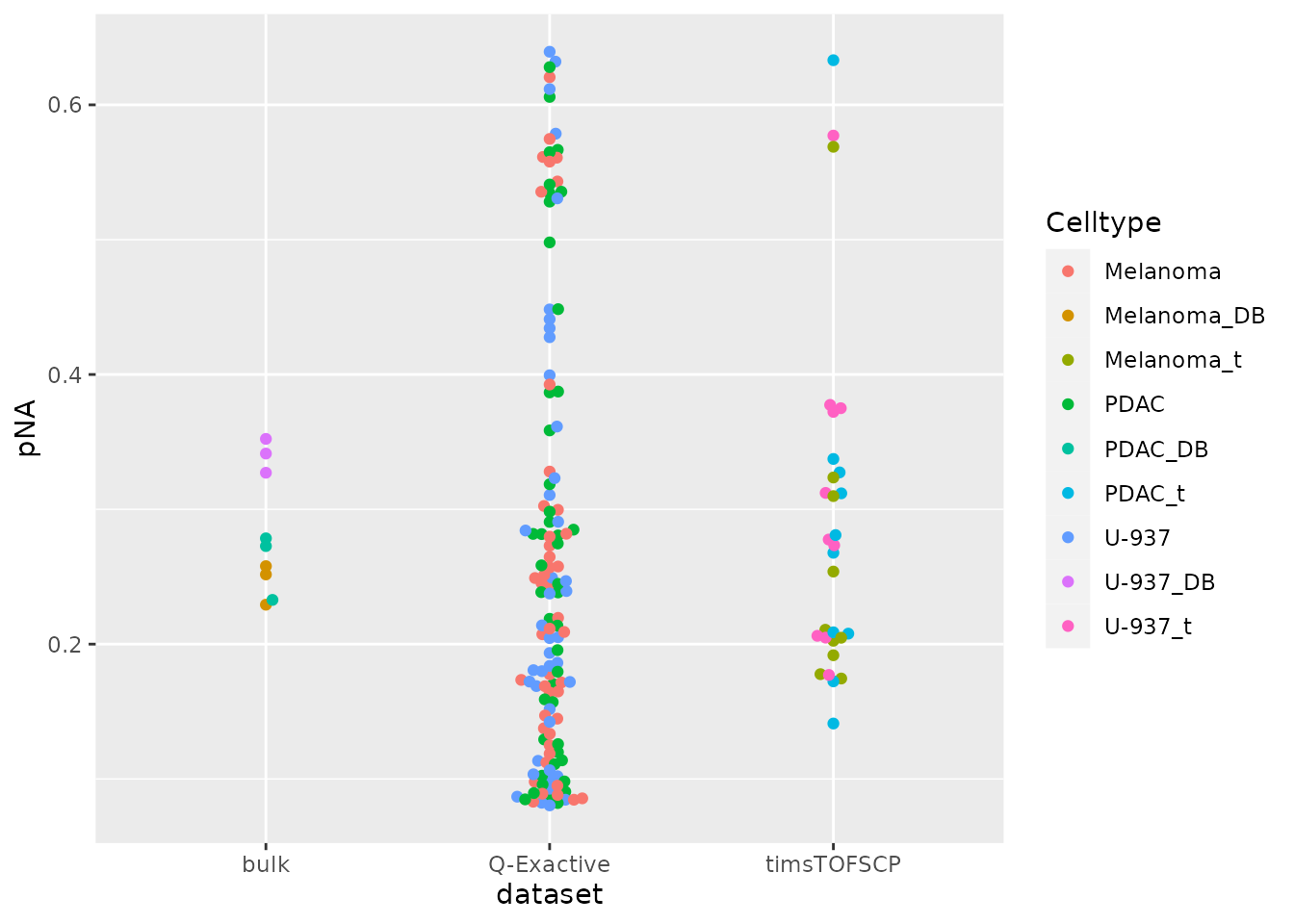
Most samples comply to the threshold. We remove the few single-cells
with too many missing data using subsetByColdata() because
we have stored pNA in the colData.
derks <- subsetByColData(derks, derks$pNA < 0.6)Clean missing data
We replace the zero values by NA’s using zeroIsNA().
derks <- zeroIsNA(derks, "prec_corrected")Batch correction
The authors then apply a first batch correction by aligning the
precursor means across the different acquisition runs. First, we extract
the combined precursor assay along with the colData using
getWithColData() and extract the quantification matrix from
it using assay()
sce <- getWithColData(derks, "prec_corrected")
## Warning: 'experiments' dropped; see 'metadata'
m <- assay(sce)
For each acquisition run, we divided each row by its mean.
for (batch in sce$File.Name) {
    ind <- which(sce$File.Name == batch)
    m[, ind] <- sweep(m[, ind, drop = FALSE], FUN = "/", MARGIN = 1,
                      STATS = rowMeans(m[, ind, drop = FALSE], na.rm = TRUE))
}
assay(sce) <- m
We add the batch corrected values as a new assay using
addAssay() and keep the links with the previous assay using
addAssayLinkOneToOne().
sce$pNA <- NULL ## Remove pNA to avoid later conflicts
derks <- addAssay(derks, sce, name = "prec_runnorm")
derks <- addAssayLinkOneToOne(derks, from = "prec_corrected", to = "prec_runnorm")
Normalization
The next step is to apply normalization. The authors perform it at the sample level and the precursor level.
Median normalize per sample
Median normalization per sample is available among the methods from
normalizeSCP(). It will automatically add a new assay that
we call prec_sampnorm
derks <- normalizeSCP(derks, "prec_runnorm", name = "prec_sampnorm",
                      method = "div.median")
Mean normalize per precursor
Mean normalization per sample is not available among the methods from
normalizeSCP(), but can be applied using
sweep() offering more flexibility.
Protein aggregation
Up to now, the data was processed at the precursor level. One protein group can be represented by several precursors. For instance, there is one protein group that is represented by over 150 precursors.
hist(table(rowData(derks[["prec_featnorm"]])$Protein.Group),
     xlab = "Number precursors per protein group", main = "")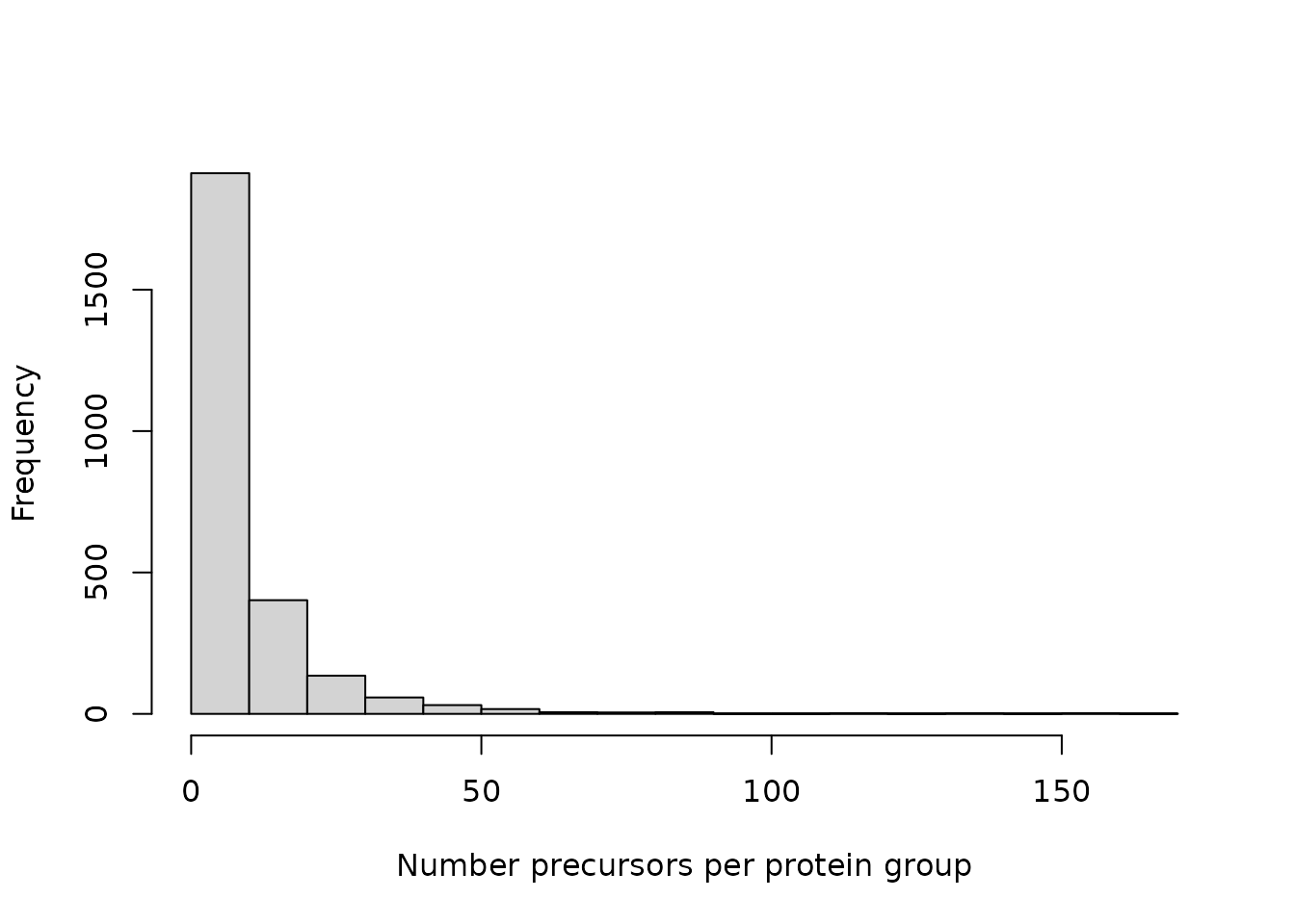
We aggregate all precursors belonging to the same protein group using
aggregateFeatures(). In this case,
fun = colMedians will assign a protein group abundance as
the median precursor abundance.
derks <- aggregateFeatures(derks, i = "prec_featnorm", name = "prot",
                           fcol = "Protein.Group", fun = colMedians,
                           na.rm = TRUE)
Batch correction
After protein agregation, the authors perform again a batch correction round. We use the same approach as above.
sce <- getWithColData(derks, "prot")
## Warning: 'experiments' dropped; see 'metadata'
## Warning: Ignoring redundant column names in 'colData(x)':
m <- assay(sce)
for (batch in sce$File.Name) {
    ind <- which(sce$File.Name == batch)
    m[, ind] <- sweep(m[, ind, drop = FALSE], FUN = "/", MARGIN = 1,
                      STATS = rowMeans(m[, ind, drop = FALSE], na.rm = TRUE))
}
assay(sce) <- m
sce$pNA <- NULL ## Remove pNA to avoid later conflicts
derks <- addAssay(derks, sce, name = "prot_runnorm")
derks <- addAssayLinkOneToOne(derks, from = "prot", to = "prot_runnorm")
Normalization
Again, the batch correction is followed by sample and protein normalization. We use the same approach as above.
derks <- normalizeSCP(derks, "prot_runnorm", name = "prot_sampnorm",
                      method = "div.median")
rowm <- rowMeans(assay(derks[["prot_sampnorm"]]), na.rm = TRUE)
derks <- sweep(derks, i = "prot_sampnorm", name = "prot_featnorm",
               MARGIN = 1, FUN = "/", STATS = rowm)
Log-transform
The protein data is log2-transformed using
logTransform().
derks <- logTransform(derks, i = "prot_featnorm", name = "prot_log",
                      base = 2)
Clean missing data
Log-transformation has generated infinite values because zeros were
present in the data. We replace these infinite values and zeros by NA’s
using infIsNA() and zeroIsNA(),
respectively.
Filter missing data
Although we already performed a first filtering based on data missingness, we further filter on protein and sample missingness.
Filter on protein missingness
We filter out proteins with more than 95% missingness. This is
performed using filterNA() that removes rows (proteins)
with a missingness higher than the given threshold.
derks <- filterNA(derks, i = "prot_log", pNA = 0.95)Imputation
Although we filtered on missing data, the protein data is majorly composed of missing values. The graph below shows the distribution of the proportion missingness in cells. Cells contain on average 65 % missing values.
data.frame(colData(derks)) %>%
    ggplot() +
    aes(y = pNA,
        x = dataset,
        color = Celltype) %>%
    geom_beeswarm()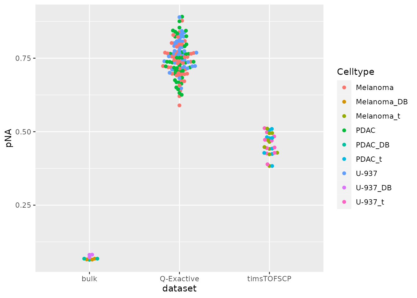
The datasets containing single-cells have more than 50% missing data
that is imputed by the authors using a custom hierarchical clustering
function. This function is available from SCP.replication
as imputeKnnSCoPE2().
derks <- imputeKnnSCoPE2(derks, i = "prot_log", name = "prot_imp", k = 3)Batch correction
A final batch correction is applied, this time using the
ComBat algorithm from the sva package.
sce <- getWithColData(derks, "prot_imp")
## Warning: 'experiments' dropped; see 'metadata'
## Warning: Ignoring redundant column names in 'colData(x)':
batch <- sce$Label
mod <- model.matrix(~ Celltype, data = colData(sce))
assay(sce) <- ComBat(assay(sce), batch = batch, mod = mod)
derks <- addAssay(derks, sce, name = "prot_bc")
derks <- addAssayLinkOneToOne(derks, from = "prot_imp", to = "prot_bc")
Normalization
Again, the batch correction is followed by sample and protein normalization. We use the same approach as above.
derks <- normalizeSCP(derks, "prot_bc", name = "prot_bc_sampnorm",
                      method = "center.median")
rowm <- rowMeans(assay(derks[["prot_bc_sampnorm"]]), na.rm = TRUE)
derks <- sweep(derks, i = "prot_bc_sampnorm", name = "prot_bc_featnorm",
               MARGIN = 1, FUN = "-", STATS = rowm)
This last normalization step leads to the final data as processed by Derks et al. We will now compare our results with the results published by the authors.
Benchmark the replication
Compare with the authors’s processed data
We first compare the data generated by the authors’s orginal script and the data generated by this vignette.
Let’s first compare the cells that were retained after processing.
allElements <- union(colnames(proteins_derks),
                     colnames(derks[["prot_bc_featnorm"]]))
table(derks2022 = allElements %in% colnames(proteins_derks),
      scp = allElements %in% colnames(derks[["prot_bc_featnorm"]]))
##          scp
## derks2022 FALSE TRUE
##     FALSE     0    7
##     TRUE      7  157
There is a good agreement between the set of filtered cells after the data processing by the authors and the data processing in this vignette.
Let’s now compare the protein groups retained after processing.
allElements <- union(rownames(proteins_derks),
                     rownames(derks[["prot_bc_featnorm"]]))
table(derks2022 = allElements %in% rownames(proteins_derks),
      scp = allElements %in% rownames(derks[["prot_bc_featnorm"]]))
##          scp
## derks2022 FALSE TRUE
##     FALSE     0  561
##     TRUE    124 1351
Most protein groups are found in both data processing workflows, but the agreement is low.
Let’s now compare the quantitative data between the two matrices. To do so, we need to intersect the column names and the rownames.
rows <- intersect(rownames(proteins_derks),
                  rownames(derks[["prot_bc_featnorm"]]))
cols <- intersect(colnames(proteins_derks),
                  colnames(derks[["prot_bc_featnorm"]]))
err <- assay(proteins_derks)[rows, cols] -
    assay(derks[["prot_bc_featnorm"]])[rows, cols]
data.frame(difference = as.vector(err[!is.na(err)])) %>%
    ggplot() +
    aes(x = difference) +
    geom_histogram(bins = 50) +
    xlab("plexDIA - scp") +
    scale_y_continuous(labels = scales::scientific) +
    theme_minimal()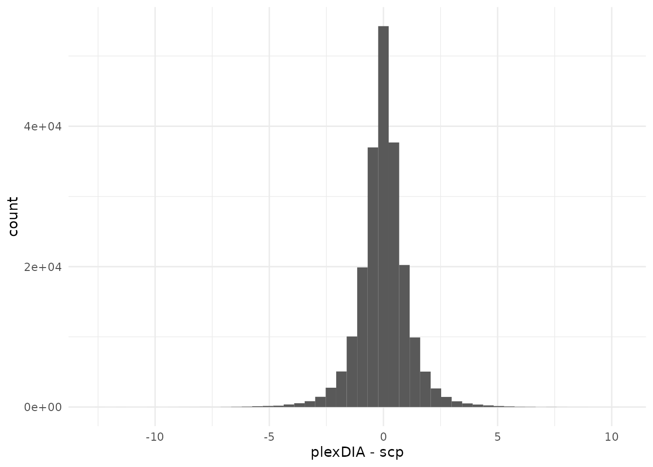
There are very large differences between the two workflows. Note that
the differences are computed on a log2 scale. However, the mode of the
distribution peaks around 0. These differences may arise because we had
to change some implementations and constraints to use our
scp framework. For instance, we had to re-implement the
isotopic carryover correction using matrix operations instead of working
with data.frames. Furthermore, as mentioned when combining
the datasets, we had to perform a consensus vote when mapping precursors
to protein groups across different datasets. These decisions taken at
the beginning may have led to small deviations from the original
workflow and may have propagated to larger deviations throughout the
data processing steps.
Number precursors per cell
We here attempt to replicate figures 6b, 6c, 6h and 6i where the
authors show the number of precursors and protein groups that were found
for each cell type in each dataset. We first compute the number of non
missing precursors per sample using countUniqueFeatures()
on the joined precursor assay, prec_corrected. The counts
are directly stored in the colData under
nprecs. Next, we do the same for the protein groups.
countUniqueFeatures() allows to group the features by a
variable of the rowData. In this case, we set
groupBy = "Protein.Groups". Note that we would get the same
results if we applied countUniqueFeatures on the
prot assay, or any protein level assay before
imputation.
derks <- countUniqueFeatures(derks, i = "prec_corrected", colDataName = "nprecs")
derks <- countUniqueFeatures(derks, i = "prec_corrected", groupBy = "Protein.Group",
                             colDataName = "nprots")
We next retrieve the counts from the `colData’ and create the plot. We perform some faceting to display precursor and protein counts for all datasets in a single panel.
df <- data.frame(colData(derks))
ggplot(df) +
    aes(x = Celltype, y = nprecs, fill = Celltype) +
    facet_wrap(~ dataset, scales = "free") +
    labs(y = "Precursors per cell") +
    ggplot(df) +
    aes(x = Celltype, y = nprots, fill = Celltype) +
    facet_wrap(~ dataset, scales = "free") +
    labs(y = "Protein groups per cell") +
    plot_layout(guides = "collect", ncol = 1) &
    geom_boxplot() &
    geom_beeswarm(alpha = 0.7) &
    xlab("") &
    theme_classic() &
    theme(legend.position = "none")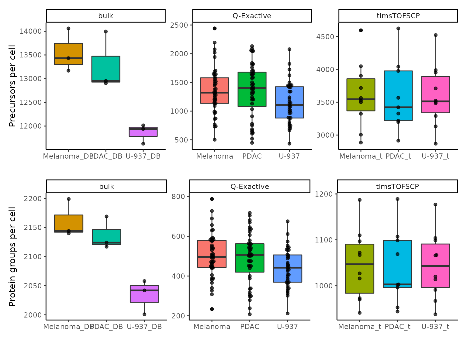
The plot is in line with the article’s figure.
Bulk vs single-cell
We here attempt to replicate figures 6f and 6l where the authors show the correlation between the PDAC vs monocyte log fold change computed from single-cell samples and from bulk samples. Although the authors devoted a separate data processing to create the plot, we here decide to keep compare single-cells and bulk using the same processing steps. We extract the processed assay, compute the fold changes between PDAC and monoyctes for the three datasets and compute the correlations between the single-cell and bulk log fold changes.
sce <- getWithColData(derks, "prot_bc_featnorm")
## Warning: 'experiments' dropped; see 'metadata'
## Warning: Ignoring redundant column names in 'colData(x)':
m <- assay(sce)
logFC <- data.frame(PvsU_tims = rowMeans(m[, sce$Celltype == "PDAC_t"], na.rm = TRUE) -
                        rowMeans(m[, sce$Celltype == "U-937_t"], na.rm = TRUE),
                    PvsU_qe = rowMeans(m[, sce$Celltype == "PDAC"], na.rm = TRUE) -
                        rowMeans(m[, sce$Celltype == "U-937"], na.rm = TRUE),
                    PvsU_bulk = rowMeans(m[, sce$Celltype == "PDAC_DB"], na.rm = TRUE) -
                        rowMeans(m[, sce$Celltype == "U-937_DB"], na.rm = TRUE),
                    Protein.Group = rownames(m))
logFC <- left_join(logFC, data.frame(Protein.Group = c("P17096;P17096-3", "P07437", "P08729"),
                                     Protein.Name = c("HMGA1", "TUBB", "KRT7")),
                   by = c("Protein.Group"))
corQE <- round(cor(logFC$PvsU_qe, logFC$PvsU_bulk,
                   use = "pairwise.complete.obs", method = "spearman"), 2)
corTims <- round(cor(logFC$PvsU_tims, logFC$PvsU_bulk,
                     use = "pairwise.complete.obs", method = "spearman"), 2)
We then plot the results as performed in the article.
ggplot(logFC) +
    aes(x = PvsU_bulk,
        y = PvsU_qe) +
    ggtitle("Q-Exactive vs Bulk", subtitle = paste0("rho = ", corQE)) +
    ggplot(logFC) +
    aes(x = PvsU_bulk,
        y = PvsU_tims) +
    ggtitle("timsTOF-SCP vs Bulk", subtitle = paste0("rho = ", corTims)) +
    plot_layout() &
    geom_pointdensity() &
    labs(x = "Log2 PDAC/U-937 100 cells",
         y = "Log2 PDAC/U-937 1 cell") &
    scale_color_continuous(type = "viridis") &
    theme_classic() &
    theme(legend.position = "none") &
    geom_label_repel(aes(label = Protein.Name),
                     min.segment.length = unit(0, 'lines'),
                     box.padding = 2,
                     size = 2.75)
## Warning: Removed 1909 rows containing missing values (geom_label_repel).
## Removed 1909 rows containing missing values (geom_label_repel).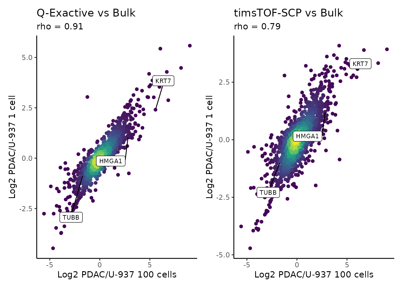
We generated a similar figure as in the article.
PCA
We now plot the PCA to reproduce Figure 6p from the author’s paper.
We use the pcaSCoPE2() function that implements the
weighted PCA as suggested in Specht et al.
(2021).
m <- assay(derks[["prot_bc_featnorm"]])
pcaRes <- pcaSCoPE2(m)
## Percent of variance explained by each principle component
pca_var <- pcaRes$values
percent_var<- pca_var/sum(pca_var)*100
## PCA scores data
pcaDf <- data.frame(PC = pcaRes$vectors[, 1:2],
                    colData(derks))
## Format the sample annotations
pcaDf$Celltype[grepl("PDAC", pcaDf$Celltype)] <- "PDAC"
pcaDf$Celltype[grepl("Mel", pcaDf$Celltype)] <- "Melanoma"
pcaDf$Celltype[grepl("^U", pcaDf$Celltype)] <- "Monocyte"
pcaDf$Label <- paste0("mTRAQ", pcaDf$Label)
We then plot the PCA results, colouring the cells either depending on the mTRAQ label used to identify tag-specific effects and depending on the cell type to illustrate the ability of the technology to capture biological variability.
ggplot(pcaDf) +
    aes(color = Label) +
    scale_color_manual(values = c("orange2","purple","turquoise")) +
    ggplot(pcaDf) +
    aes(color = Celltype) +
    scale_color_manual(values = c("#52B788","#457B9D","#E07A5F")) +
    plot_annotation(title = "PCA of the processed data using 'scp'",
                    subtitle = paste0(sum(pcaDf$dataset != "Bulk"), " cells\n",
                                      nrow(m), " protein groups")) +
    plot_layout(guides = "collect") &
    aes(x = PC.1,
        y = PC.2,
        size = dataset,
        shape = dataset,
        alpha = dataset) &
    geom_point(alpha = 0.66) &
    labs(x = paste0("PC1 (", round(percent_var[1],0),"%)"),
         y = paste0("PC2 (", round(percent_var[2],0),"%)")) &
    scale_size_manual(values = c(5, 2, 2)) &
    theme_classic()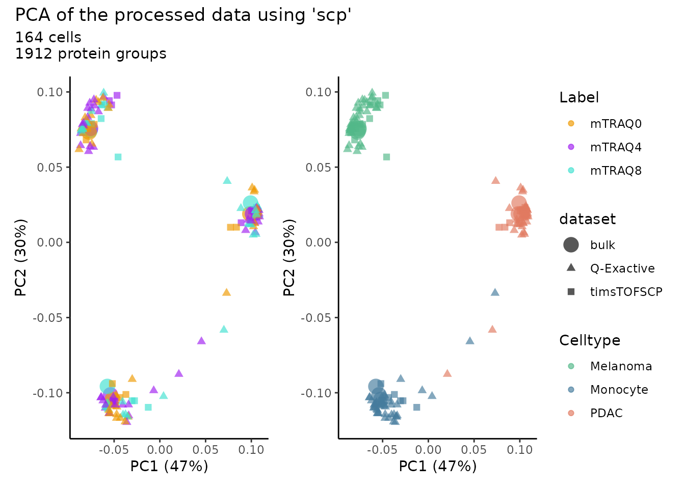
Although the we could not accurately replicate the data provided by the authors, we can clearly see the same global pattern as in the original work.
Reproduce this vignette
You can reproduce this vignette using Docker:
docker pull cvanderaa/scp_replication_docker:v1
docker run \
    -e PASSWORD=bioc \
    -p 8787:8787 \
    cvanderaa/scp_replication_docker:v1
Open your browser and go to http://localhost:8787. The USER is rstudio
and the password is bioc. You can find the vignette in the
vignettes folder.
See the website home page for more information.
Requirements
Hardware and software
The system details of the machine that built the vignette are:
## Machine: Linux (5.15.0-48-generic)
## R version: R.4.2.1 (svn: 82513)
## RAM: 16.5 GB
## CPU: 16 core(s) - 11th Gen Intel(R) Core(TM) i7-11800H @ 2.30GHzSession info
sessionInfo()
## R version 4.2.1 (2022-06-23)
## Platform: x86_64-pc-linux-gnu (64-bit)
## Running under: Ubuntu 20.04.4 LTS
##
## Matrix products: default
## BLAS:   /usr/lib/x86_64-linux-gnu/blas/libblas.so.3.9.0
## LAPACK: /usr/lib/x86_64-linux-gnu/lapack/liblapack.so.3.9.0
##
## locale:
##  [1] LC_CTYPE=en_US.UTF-8       LC_NUMERIC=C
##  [3] LC_TIME=en_US.UTF-8        LC_COLLATE=en_US.UTF-8
##  [5] LC_MONETARY=en_US.UTF-8    LC_MESSAGES=en_US.UTF-8
##  [7] LC_PAPER=en_US.UTF-8       LC_NAME=C
##  [9] LC_ADDRESS=C               LC_TELEPHONE=C
## [11] LC_MEASUREMENT=en_US.UTF-8 LC_IDENTIFICATION=C
##
## attached base packages:
## [1] stats4    stats     graphics  grDevices utils     datasets  methods
## [8] base
##
## other attached packages:
##  [1] benchmarkme_1.0.8           ggpointdensity_0.1.0
##  [3] patchwork_1.1.2             ggrepel_0.9.1
##  [5] ggbeeswarm_0.6.0            forcats_0.5.2
##  [7] stringr_1.4.1               dplyr_1.0.10
##  [9] purrr_0.3.4                 readr_2.1.3
## [11] tidyr_1.2.1                 tibble_3.1.8
## [13] ggplot2_3.3.6               tidyverse_1.3.2
## [15] sva_3.45.0                  BiocParallel_1.31.12
## [17] genefilter_1.79.0           mgcv_1.8-40
## [19] nlme_3.1-159                SCP.replication_0.2.1
## [21] SingleCellExperiment_1.19.1 scpdata_1.5.4
## [23] ExperimentHub_2.5.0         AnnotationHub_3.5.2
## [25] BiocFileCache_2.5.0         dbplyr_2.2.1
## [27] scp_1.7.4                   QFeatures_1.7.3
## [29] MultiAssayExperiment_1.23.9 SummarizedExperiment_1.27.3
## [31] Biobase_2.57.1              GenomicRanges_1.49.1
## [33] GenomeInfoDb_1.33.7         IRanges_2.31.2
## [35] S4Vectors_0.35.4            BiocGenerics_0.43.4
## [37] MatrixGenerics_1.9.1        matrixStats_0.62.0
## [39] BiocStyle_2.25.0
##
## loaded via a namespace (and not attached):
##   [1] readxl_1.4.1                  backports_1.4.1
##   [3] BiocBaseUtils_0.99.12         systemfonts_1.0.4
##   [5] igraph_1.3.5                  lazyeval_0.2.2
##   [7] splines_4.2.1                 digest_0.6.29
##   [9] foreach_1.5.2                 htmltools_0.5.3
##  [11] fansi_1.0.3                   magrittr_2.0.3
##  [13] memoise_2.0.1                 doParallel_1.0.17
##  [15] googlesheets4_1.0.1           cluster_2.1.4
##  [17] tzdb_0.3.0                    limma_3.53.10
##  [19] Biostrings_2.65.6             annotate_1.75.0
##  [21] modelr_0.1.9                  pkgdown_2.0.6
##  [23] colorspace_2.0-3              rvest_1.0.3
##  [25] blob_1.2.3                    rappdirs_0.3.3
##  [27] textshaping_0.3.6             haven_2.5.1
##  [29] xfun_0.33                     crayon_1.5.2
##  [31] RCurl_1.98-1.9                jsonlite_1.8.2
##  [33] iterators_1.0.14              survival_3.4-0
##  [35] glue_1.6.2                    gtable_0.3.1
##  [37] gargle_1.2.1                  zlibbioc_1.43.0
##  [39] XVector_0.37.1                OrgMassSpecR_0.5-3
##  [41] DelayedArray_0.23.2           scales_1.2.1
##  [43] DBI_1.1.3                     edgeR_3.39.6
##  [45] Rcpp_1.0.9                    viridisLite_0.4.1
##  [47] xtable_1.8-4                  clue_0.3-61
##  [49] reticulate_1.26               bit_4.0.4
##  [51] MsCoreUtils_1.9.1             httr_1.4.4
##  [53] ellipsis_0.3.2                farver_2.1.1
##  [55] pkgconfig_2.0.3               XML_3.99-0.11
##  [57] sass_0.4.2                    here_1.0.1
##  [59] locfit_1.5-9.6                utf8_1.2.2
##  [61] labeling_0.4.2                tidyselect_1.1.2
##  [63] rlang_1.0.6                   later_1.3.0
##  [65] AnnotationDbi_1.59.1          munsell_0.5.0
##  [67] BiocVersion_3.16.0            cellranger_1.1.0
##  [69] tools_4.2.1                   cachem_1.0.6
##  [71] cli_3.4.1                     generics_0.1.3
##  [73] RSQLite_2.2.17                broom_1.0.1
##  [75] evaluate_0.16                 fastmap_1.1.0
##  [77] yaml_2.3.5                    ragg_1.2.3
##  [79] knitr_1.40                    bit64_4.0.5
##  [81] fs_1.5.2                      KEGGREST_1.37.3
##  [83] AnnotationFilter_1.21.0       mime_0.12
##  [85] xml2_1.3.3                    compiler_4.2.1
##  [87] beeswarm_0.4.0                filelock_1.0.2
##  [89] curl_4.3.2                    png_0.1-7
##  [91] interactiveDisplayBase_1.35.0 reprex_2.0.2
##  [93] bslib_0.4.0                   stringi_1.7.8
##  [95] highr_0.9                     desc_1.4.2
##  [97] lattice_0.20-45               ProtGenerics_1.29.0
##  [99] Matrix_1.5-1                  vctrs_0.4.2
## [101] pillar_1.8.1                  lifecycle_1.0.2
## [103] BiocManager_1.30.18           jquerylib_0.1.4
## [105] bitops_1.0-7                  httpuv_1.6.6
## [107] R6_2.5.1                      bookdown_0.29
## [109] promises_1.2.0.1              vipor_0.4.5
## [111] codetools_0.2-18              benchmarkmeData_1.0.4
## [113] MASS_7.3-58.1                 assertthat_0.2.1
## [115] rprojroot_2.0.3               withr_2.5.0
## [117] GenomeInfoDbData_1.2.9        parallel_4.2.1
## [119] hms_1.1.2                     grid_4.2.1
## [121] rmarkdown_2.16                googledrive_2.0.0
## [123] lubridate_1.8.0               shiny_1.7.2
Licence
This vignette is distributed under a CC BY-SA licence licence.