Chapter 3 High-level data structures
Learning objectives
- Understand the difference between basic data structures and high-level objects.
- Understand the concept of high-level object.
- Know how to learn about objects and access data from them.
- Learn about how to import Bioconductor objects widely used in omics data analysis.
- Become familiar with how objects are implemented.
3.1 Introduction
The term object stems from the widely used object-oriented programming (OOP) paradigm. OOP is however outside of scope of this course (see part III of Wickham (2014Wickham, Hadley. 2014. Advanced R. Chapman & Hall/CRC the r Series. Taylor & Francis.), which is also freely available online). In the R refresher chapter 1, we have seen the base types of R, which we have efficiently used in many situations. Sometimes, however, these aren’t enough.
We have also use object, for example in chapter 2, when
generating ggplot visualisation. We have seen that it is possible to
store the output of ggplot2 in a variable, that contain all the data
and information necessary to produce the figure.
3.2 Why objects?
Combine many parts of a complex data, for example store data (and possibly different forms thereof (see chapter 5) and metadata together.
Objects are self describing: an object to store high-throughput sequencing (HTS) data contains high-throughput sequencing data. Replace high-throughput sequencing data by DNA sequences (see chapter 4), proteomics, … and it will still hold.
Using object enables consistency3 This consistency comes however at the cost of flexibility, hence the importance of well designed objects, that fit several use cases for the type of data at hand.: whoever prepares the HTS data, it will always have the same structure.
- If all information is stored in a single object4 This idea is consistent with the notion that you would like to place all the data relevant to an expriment into a single folder., it is easier to save it, to share it with others, and to use it as an input to a function.
The above properties lead to greater robustness and interoperability when working with objects modelling complex data.
Common behaviour (methods) can be specialised to match the particular data type (this is called polymorphism): for example plotting (a vector, a matrix, NGS data), summary, subsetting (
[and[[), …Another import benefit of using objects to model complex data is abstraction: it is possible to hide all the (unnecessary for its usage) complexity of a particular type of data and present/give access to its most imporant parts in a user-friendly interface and efficient way.
Relations between object can be recorded (this is called inheritance).
To avoid confusion, it is useful to define and separate objects and classes. A class describes (models) the general properties for groups of objects. For example, we could define a class to describe people in this course as follows:
Class person:
- Name: a character
- Surname: a character
- Noma: an optional numeric
- Role: a character (student, teaching assistant, instructor)
An object is an instantiation of a class with specific values in its fields:
Object of class person:
- Name: Laurent
- Surname: Gatto
- Noma: NA
- Role: instructor
► Question
Write down two objects that would describe a teaching assistant and a student.
► Solution
We will focus on objects and their usage here.
3.3 Examples in base R
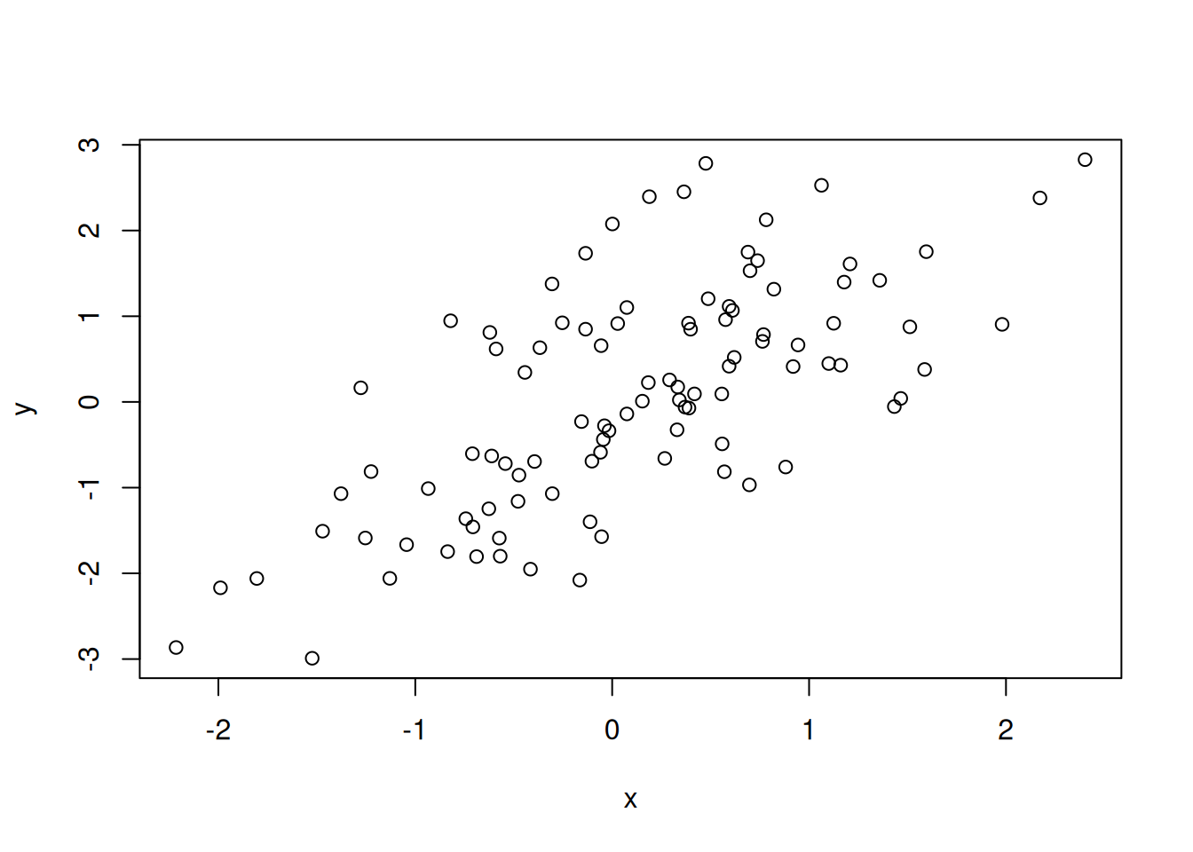
Let’s start by generating a testing dataset composed of two correlated
variables, x and y:
##            x          y
## 1 -0.6264538 -1.2468205
## 2  0.1836433  0.2257592
## 3 -0.8356286 -1.7465503
## 4  1.5952808  1.7533096
## 5  0.3295078 -0.3250769
## 6 -0.8204684  0.9468189
Figure 3.1: The x and y variables display a linear relationship.
We are now going to model the linear relation between x and y
using the lm (linear model) function. The resulting variable fit
is the result of computing the linear regression
\(y = \beta_{0} + \beta_{1} x + \epsilon\).
When printing the object, we see the call we performed, the
intercept (\(\beta_0\)) and the slope (\(\beta_1\)) of the regression.
##
## Call:
## lm(formula = y ~ x, data = df)
##
## Coefficients:
## (Intercept) x
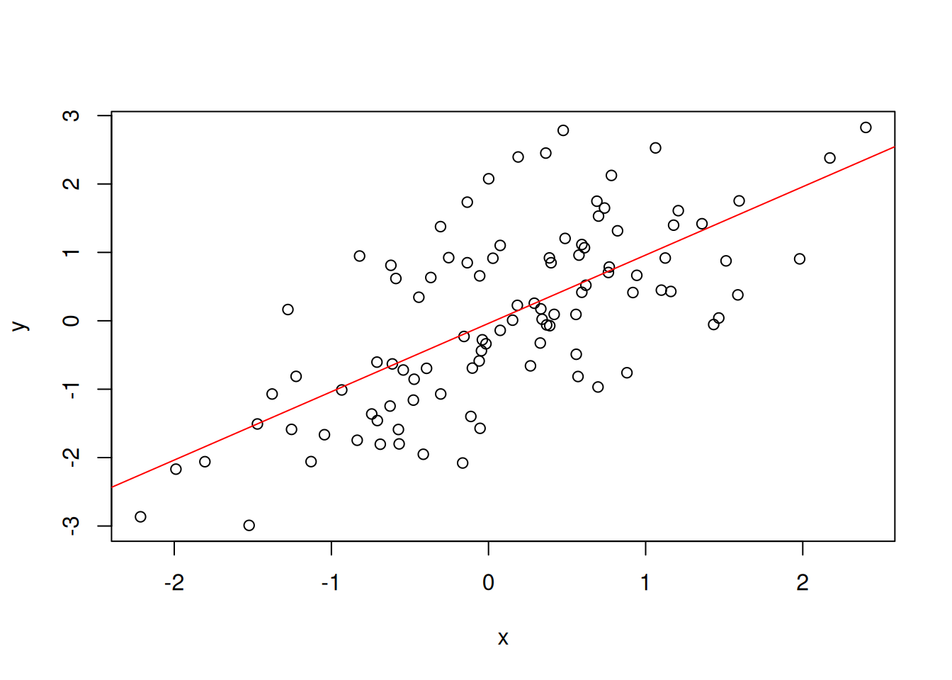
## -0.03769 0.99894We can plot the linear regression line with abline and passing the
fit variable.
Figure 3.2: The regression line modelling the linear regression between the two x and y variables.
The fit variable is an object of class lm, which we can check with
the class function.
## [1] "lm"It contains much more than simply the intercept and the slope of the regression line.
► Question
Find out what an object of class lm contains by exploring the
content of the fit object (try the names and str functions) and
reading the lm manual page.
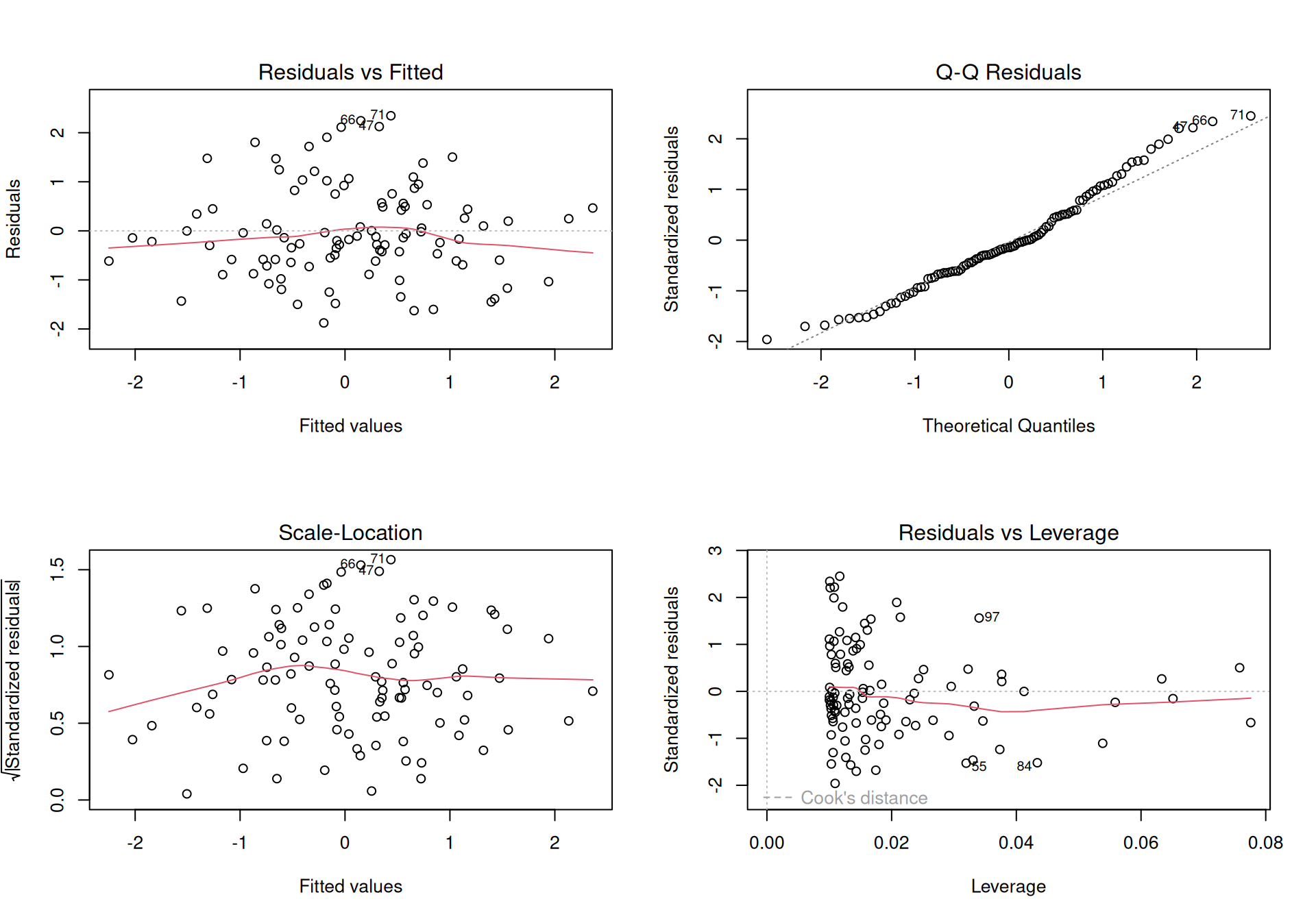
Finally, to demonstrate polymorphism, let’s try to plot the fit
variable.
Figure 3.3: Plotting an instance of class lm produces a set of diagnostic plots, that inform us about the quality of the regression.
3.4 Examples from the Bioconductor project
We have already briefly seen the Bioconductor project. It initiated by Robert Gentleman (Gentleman et al. (2004Gentleman, Robert C., Vincent J. Carey, Douglas M. Bates, Ben Bolstad, Marcel Dettling, Sandrine Dudoit, Byron Ellis, et al. 2004. “Bioconductor: Open Software Development for Computational Biology and Bioinformatics.” Genome Biol 5 (10): –80. https://doi.org/10.1186/gb-2004-5-10-r80.); Huber et al. (2015Huber, W, V J Carey, R Gentleman, S Anders, M Carlson, B S Carvalho, H C Bravo, et al. 2015. “Orchestrating High-Throughput Genomic Analysis with Bioconductor.” Nat Methods 12 (2): 115–21. https://doi.org/10.1038/nmeth.3252.)), one of the two creators of the R language, and centrally offers dedicated R packages for bioinformatics.
Bioconductor provides tools for the analysis and comprehension of high-throughput genomic data. Bioconductor uses the R statistical programming language, and is open source and open development. It has two releases each year, and an active user community.
This video provides a great overview of the project at large.
Bioconductor provides a rich set of classes for omics data, summarised below.
3.4.1 Common Bioconductor classes
- Rectangular feature x sample data – SummarizedExperiment
::SummarizedExperiment()(RNAseq count matrix, microarray, …) - Genomic coordinates – GenomicRanges
::GRanges()(1-based, closed interval) - DNA / RNA / AA sequences – Biostrings
::*StringSet() - Gene sets – GSEABase
::GeneSet()GSEABase::GeneSetCollection() - Multi-omics data – MultiAssayExperiment
::MultiAssayExperiment() - Single cell data – SingleCellExperiment
::SingleCellExperiment() - Mass spectrometry data – Spectra
::Spectra() - Quantitative proteomics data – QFeatures
::QFeatures()
3.4.2 The SummarizedExperiment class
Let’s start by installing5 Before installing the package, we first check if they are
available with require. If they are missing, the call to
require will return FALSE, otherwise it returns TRUE and
loads the packages. Given that we negate the return value of
require using !, the packages will be installed only when
missing. theSummarizedExperiment
package, that implements the class, and the airway
data package, that provides an RNA-Seq example data.
if (!require("SummarizedExperiment"))
    BiocManager::install("SummarizedExperiment")
if (!require("airway"))
    BiocManager::install("airway")
If you know you have the packages, it is more straightforward to directly load the packages.
The airway package provides a data for an RNA-Seq experiment on four
human airway smooth muscle cell lines treated with dexamethason
published by Himes et al. (2014Himes, B E, X Jiang, P Wagner, R Hu, Q Wang, B Klanderman, R M Whitaker, et al. 2014. “RNA-Seq Transcriptome Profiling Identifies CRISPLD2 as a Glucocorticoid Responsive Gene That Modulates Cytokine Function in Airway Smooth Muscle Cells.” PLoS One 9 (6): e99625. https://doi.org/10.1371/journal.pone.0099625.). It contains the RNA expression data for
64102 transcripts and 8 samples. These 8 samples correspond to treated
and untreated condition in 4 different cell lines.
Objects of the class SummarizedExperiment contain one or more assays
(i.e. sets if quantitative expresson data), each represented by a
matrix-like object (typically) of numeric mode. The rows represent
features such as genes, transcripts, proteins or more generally
genomic ranges and the columns represent samples. The figure below
represents its anatomy in greater details.
Figure 3.4: Schematic representation of the anatomy if a SummarizedExperiment object. (Figure taken from the SummarizedExperiment package vignette.)

- The sample (columns) metadata can be accessed with the
colData()function. - The features (rows) metadata can be accessed with the
rowData()column. - If the features represent ranges along genomic coordinates, these
can be accessed with
rowRanges() - Additional metadata describing the overall experiment can be
accessed with
metadata(). - The quantiative data can be accessed with
assay(). -
assays()returns a list of matrix-like assays.
► Question
Load the airway data and display it in your R console. Make sure you
understand all parts in the short text summary that is displayed. What
class is airway of.
► Question
Extract the quantitative assay data, the rows and columns metadata,
the row ranges and the experiment metadata. What are the classes of
these individual parts of the SummarizedExperiment object.
► Solution
The row and column metadata are stored as a special data.frame
implementation6 Like the tibble, that is an implememtation specific to the
tidyverse packages., that has been developed in the Bioconductor
project. It behaves like like a classical data.frame.
► Question
What biological sample names in the airway dataset were treated with
dexamethason? Which ones weren’t?
► Solution
► Question
What are the dimensions of the assay data, and the row and column metadata? What can you way about these?
► Solution
3.4.3 Subsetting SummarizedExperiment objects
As mentioned in the introduction, it is possible to redefine common
functions to have a special behaviour with objects. This is the case
for the [ operator, that will automatically subset all parts of the
object. Below, we create a new instance of class
SummarizedExperiment that contains only the 5 first features for the
3 first samples.
## class: RangedSummarizedExperiment
## dim: 5 3
## metadata(1): ''
## assays(1): counts
## rownames(5): ENSG00000000003 ENSG00000000005 ENSG00000000419
##   ENSG00000000457 ENSG00000000460
## rowData names(10): gene_id gene_name ... seq_coord_system symbol
## colnames(3): SRR1039508 SRR1039509 SRR1039512
## colData names(9): SampleName cell ... Sample BioSample
► Question
Verfiy that the assay data, the column and row metadata and the row ranges have been preserved.
Subsetting can be performed with numeric vectors (as shown above), as well as character of logical vectors, just like with dataframes or matrices.
► Question
Create a new object that contains the data for features (rows)
"ENSG00000166963", "ENSG00000267970" and "ENSG00000254663" and
samples (columns) "SRR1039517" and "SRR1039521".
► Solution
The row ranges are defined as a list of genomic ranges (GRanges
objects), one genomic range per row in the
SummarizedExperiment. This GRangesList object behaves like a list,
albeit a list that specifically contains GRanges objects.
If we look at the first feature, corresponding to gene
ENSG00000000003, we see that is is composed of 17 exons
(ENSE00001459322 to ENSE00001828996) and their detailed positions
on chromosome X.
## GRanges object with 17 ranges and 2 metadata columns:
##        seqnames            ranges strand |   exon_id       exon_name
##           <Rle>         <IRanges>  <Rle> | <integer>     <character>
##    [1]        X 99883667-99884983      - |    667145 ENSE00001459322
##    [2]        X 99885756-99885863      - |    667146 ENSE00000868868
##    [3]        X 99887482-99887565      - |    667147 ENSE00000401072
##    [4]        X 99887538-99887565      - |    667148 ENSE00001849132
##    [5]        X 99888402-99888536      - |    667149 ENSE00003554016
##    ...      ...               ...    ... .       ...             ...
##   [13]        X 99890555-99890743      - |    667156 ENSE00003512331
##   [14]        X 99891188-99891686      - |    667158 ENSE00001886883
##   [15]        X 99891605-99891803      - |    667159 ENSE00001855382
##   [16]        X 99891790-99892101      - |    667160 ENSE00001863395
##   [17]        X 99894942-99894988      - |    667161 ENSE00001828996
##   -------
##   seqinfo: 722 sequences (1 circular) from an unspecified genome
The position of genes can also be used to subset a
SummarizedExperiment. In the example below, we select all features
that overlap with positions 100000 to 1100000 on chromosome 1. To do
this we first create a new GRanges object that matches the region of
interest:
## GRanges object with 1 range and 0 metadata columns:
##       seqnames         ranges strand
##          <Rle>      <IRanges>  <Rle>
##   [1]        1 100000-1100000      *
##   -------
##   seqinfo: 1 sequence from an unspecified genome; no seqlengths
We can now use roi to extract the feature of interest with the
subsetByOverlaps function, which returns a new
SummarizedExperiment object that contains 74 features.
## class: RangedSummarizedExperiment
## dim: 74 8
## metadata(1): ''
## assays(1): counts
## rownames(74): ENSG00000131591 ENSG00000177757 ... ENSG00000272512
##   ENSG00000273443
## rowData names(10): gene_id gene_name ... seq_coord_system symbol
## colnames(8): SRR1039508 SRR1039509 ... SRR1039520 SRR1039521
## colData names(9): SampleName cell ... Sample BioSample
► Question
How many genes are present on chromosome X between position 100000 et 1000000.
► Solution
► Question
Visit the Ensembl page and look up the Ensembl gene identifier
(ENSG00...) of the BRCA1 gene. Verify if these match the information
in the airway data. If not, why could this be? How many exons are
there in the airway data for this gene?
► Solution
3.4.4 Constructing a SummarizedExperiment
Complex object such as SummarizedExperiment are generally
constructed by functions (called constructors) from files. It is
possible to construct a SummarizedExperiment by hand. To do so, we
first need to construct the different parts of the object.
Let’s create an expression matrix for 200 genes and 6 samples by randomly sample values between 1 and 10000.
Below, we create a the colData part using the appropriate
constructor for the class of data needed:
Let’s also create some ranges. Here, we will have one range per
features, as opposed to the airway data, that has multiple ranges
(exons) per feature (gene). The ranges below to chromosomes 1 and 2
(50 and 150 respectively), with ranges (constructure with the
IRanges constructor) starting between 1e5 and 1e6 with width 100,
and strand chosing randomly as the positive or negative strand.
rng <- GRanges(seqnames = rep(c("chr1", "chr2"), c(50, 150)),
               ranges = IRanges(floor(runif(200, 1e5, 1e6)), width = 100),
               strand = sample(c("+", "-"), 200, TRUE))
We can now put the different parts together using the
SummarizedExperiment constructor:
## class: RangedSummarizedExperiment
## dim: 200 6
## metadata(0):
## assays(1): counts
## rownames: NULL
## rowData names(0):
## colnames(6): A B ... E F
## colData names(1): Treatment
We can also create a rowData object and add it to our se object:
## class: RangedSummarizedExperiment
## dim: 200 6
## metadata(0):
## assays(1): counts
## rownames: NULL
## rowData names(1): some_value
## colnames(6): A B ... E F
## colData names(1): Treatment
3.5 Additional exercises
► Question
Using the function kem2.tsv from the rWSBIM1207 package, import
the count and annotation data into R and use them to create an object
of class SummarizedExperiment.
Page built: 2026-03-31 using R version 4.5.0 (2025-04-11)