Chapter 9 Bioinformatics
As already alluded to earlier, Wikipedia defines bioinformatics as
Bioinformatics is an interdisciplinary field that develops methods and software tools for understanding biological data.
Bioinformatics is as varied as biology itself, and ranges from data analysis, to software development, computational or statistical methodological development, more theoretical work, as well as any combination of these.
9.1 Omics data
So far, we have explored broad data science techniques in R. A widespread and successful area of bioinformatics, and one that you, as a biology or biomedical science student are likely to be confronted with, is the analysis and interpretation of omics data.
).](figs/Centraldogma_nodetails.png) Figure 9.1: Information flow in biological systems (Source Wikipedia).
Figure 9.1: Information flow in biological systems (Source Wikipedia).
It is useful to define these omics data along the flow of information in biology (Figure 9.1), and define the different application domains. The technologies that focus on DNA, and the genome in particular (either whole or parts thereof) are termed genomics, and are currently based on sequencing, in particular high throughput sequencing (HTS). The domain focusing on the study of any DNA (or associated proteins) modification (such as for example methylation) is termed epigenetics. The study of RNA, and more specifically the quantitation of RNA levels in biological samples is termed transcriptomics, as it assays the transcription of DNA into RNA molecules. Without further specification, transcriptomics refers to the quantitation of message RNA, although one could also focus on non-coding RNAs such as micro RNAs. HTS is currently the technology of choice for any transcriptomics study, while a decade ago, prior to the development of RNA sequencing (called RNA-Seq), microarrays were widely used. Proteomics focuses on the identification and quantitation of proteins, and can also expand into the study of protein interactions, post-translational modifications or sub-cellular localisation of proteins. Further downstream of proteins, small molecules or lipids can also be assayed under the umbrella terms of metabolomics and lipidomics. The technology of choice for protein, lipids or smaller metabolites is mass spectrometry.
In the next couple of sections, some important concepts related to omics data and their analysis are repeated and emphasised.
High throughput
By it very nature, omics data is high throughput. The goal is to measure all, or as many as possible molecules of an omics-domain as possible: sequence the whole genome or all exomes; identify all epigenetic histone modifications (defining the compactness of DNA and hence it’s accessibility by the transcription machinery); identify and quantify as much as possible from the complete proteomics; etc. As a result, omics data is both large in size and complex in nature, and requires dedicated software and analysis methods to be processed, analysed to infer biologically relevant patterns.
Raw and processed data
The omics data that are produced by the instruments are called raw data, and their size (generally large), the types of file, and structure will depend on the technology that is used. Raw data need to be processed using dedicated software before obtaining data that can be mapped to the biology that is measured. Below we illustrate two such examples using Sanger sequencing and mass spectrometry.
In Sanger sequencing (Figure 9.2), DNA is labelled using fluorophores, and different nucleotides are marked with different colours. Upon acquisition, light signal is acquired and recording of the different colours can be used to reconstruct the DNA sequence.
Figure 9.2: Processing Sanger sequencing data to a string. (Source BiteSizeBio).
).](figs/sanger-sequencing.jpg)
In mass spectrometry, charged molecules are separated based on their mass-to-charge (M/Z) ratio and their intensities recorded to produce a spectrum. In proteomics, the molecules that are assayed are protein fragments called peptides. Upon fragmentation of peptides, the different between the M/Z peaks of the peptide fragment ions can be used to reconstruct the peptide sequence (Figure 9.3).
Figure 9.3: De novo peptide sequencing using mass spectrometry. (Source Creative Proteomics).
).](figs/de-novo-pep-sequencing.jpg)
The size and computational cost of processing raw data often require more serious hardware, including disk space, computer clusters with 100s or more of compute nodes and/or access to high amounts of memory (RAM).
Processed data themselves often need to be further transformed to account for a variety of noise that is inherent to sample collection, preparation and measurement acquisition. Data processing and transformation will be explored in detail in subsequent course such as Omics data analysis (WSBIM2122).
9.2 Metadata and experimental design
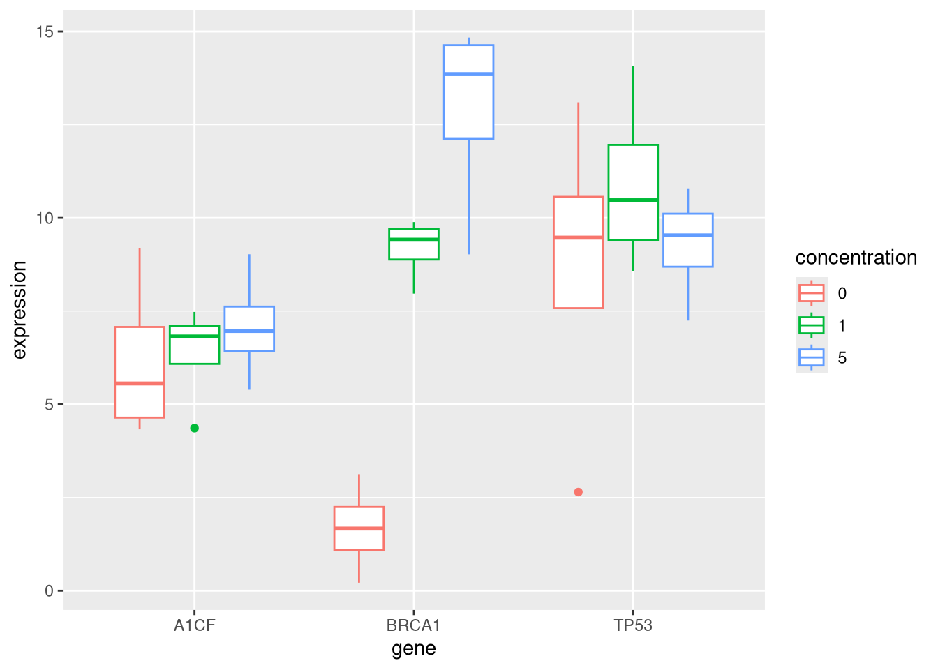
The acquired data, even once processed, is still of very little use when it comes to understanding biology. Before samples are collected and data are generated, it is essential to carefully design a question of interest (research hypothesis) and the experiment that will allow to answer it. For example, if we want to understand the effect of a particular drug on cancer cells, and more specifically understand the effect on the transcription of all the expressed genes, on would need to measure gene expression (using for example RNA-Seq) in cancer cells in presence and absence of that drug. The table below describes a simple experimental design where 3 conditions (control, drug at a concentrations of 1 and 5) have been simultaneously processed and measured by the same operator in 4 replicate.
| sample | operator | date | group | concentration | replicate |
|---|---|---|---|---|---|
| S1 | Kevin | 2019-03-02 | CTRL | 0 | 1 |
| S2 | Kevin | 2019-03-02 | CTRL | 0 | 2 |
| S3 | Kevin | 2019-03-02 | CTRL | 0 | 3 |
| S4 | Kevin | 2019-03-02 | CTRL | 0 | 4 |
| S5 | Kevin | 2019-03-02 | DRUG | 1 | 1 |
| S6 | Kevin | 2019-03-02 | DRUG | 1 | 2 |
| S7 | Kevin | 2019-03-02 | DRUG | 1 | 3 |
| S8 | Kevin | 2019-03-02 | DRUG | 1 | 4 |
| S9 | Kevin | 2019-03-02 | DRUG | 5 | 1 |
| S10 | Kevin | 2019-03-02 | DRUG | 5 | 2 |
| S11 | Kevin | 2019-03-02 | DRUG | 5 | 3 |
| S12 | Kevin | 2019-03-02 | DRUG | 5 | 4 |
We have seen a much more complex experimental design, involving many
more samples with the clinical1 data.
## # A tibble: 516 × 15
##    patientID    tumor_tissue_site gender age_at_diagnosis vital_status
##    <chr>        <chr>             <chr>             <int>        <int>
##  1 TCGA-05-4249 lung              male              24532            0
##  2 TCGA-05-4382 lung              male              24868            0
##  3 TCGA-05-4384 lung              male              24411            0
##  4 TCGA-05-4389 lung              male              25660            0
##  5 TCGA-05-4390 lung              female            21430            0
##  6 TCGA-05-4395 lung              male              27971            1
##  7 TCGA-05-4396 lung              male              28094            1
##  8 TCGA-05-4398 lung              female            17471            0
##  9 TCGA-05-4402 lung              female            20819            1
## 10 TCGA-05-4403 lung              male              27881            0
## # ℹ 506 more rows
## # ℹ 10 more variables: days_to_death <int>, days_to_last_followup <int>,
## #   pathologic_stage <chr>, pathology_T_stage <chr>, pathology_N_stage <chr>,
## #   pathology_M_stage <chr>, smoking_history <chr>,
## #   number_pack_years_smoked <dbl>, year_of_tobacco_smoking_onset <int>,
## #   stopped_smoking_year <int>
When performing experiments, measurements should also be repeated several times (typically at least three), to quantify the overall variability (technical and biological) in the measured variables and, eventually, identify changes that relate to the conditions of interest (for example differences in genes expression in the presence or absence of the drug).
Figure 9.4: Distribution of the expression of the genes A1CF, BRCA1 and TP53 under the control (no drug) and drug at concentrations 1 and 5.
9.3 The Bioconductor project
The Bioconductor was initiated by Robert Gentleman (R. C. Gentleman et al. (2004Gentleman, Robert C., Vincent J. Carey, Douglas M. Bates, Ben Bolstad, Marcel Dettling, Sandrine Dudoit, Byron Ellis, et al. 2004. “Bioconductor: Open Software Development for Computational Biology and Bioinformatics.” Genome Biol 5 (10): –80. https://doi.org/10.1186/gb-2004-5-10-r80.);Huber et al. (2015Huber, W, V J Carey, R Gentleman, S Anders, M Carlson, B S Carvalho, H C Bravo, et al. 2015. “Orchestrating High-Throughput Genomic Analysis with Bioconductor.” Nat Methods 12 (2): 115–21. https://doi.org/10.1038/nmeth.3252.)), one of the two creators of the R language, and centrally offers dedicated R packages for bioinformatics.
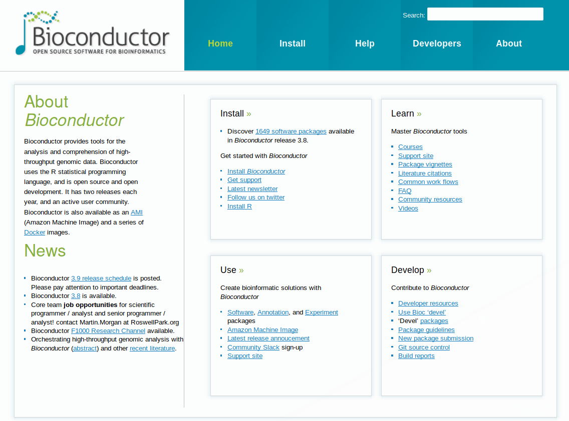
Bioconductor provides tools for the analysis and comprehension of high-throughput genomic data. Bioconductor uses the R statistical programming language, and is open source and open development. It has two releases each year, and an active user community.
Figure 9.5: The Bioconductor web page.
This video provides a great overview of the project at large.
Bioconductor packages are managed installed using a dedicated package,
namely BiocManager, that can be installed from CRAN with
Individuals package such as SummarizedExperiment (see below for
details), DESeq2 (for transcriptomics), Spectra (for mass
spectrometry), xcms (metabolomics), … can then be installed with
BiocManager::install.
BiocManager::install("SummarizedExperiment")
BiocManager::install("DESeq2")
BiocManager::install("Spectra")
BiocManager::install("xcms")
Note that we can also use that same function to install packages from GitHub:
9.4 Omics data containers
Data in bioinformatics is often more complex than the basic data types we have seen so far. In such situations, developers define specialised data containers (termed classes that) that match the properties of the data they need to handle.
An example of general data architecture, that is used across many omics domains in Bioconductor is represented below:
Figure 9.6: A data structure to store quantitative data, features (rows) annotation, and samples (column) annotations..
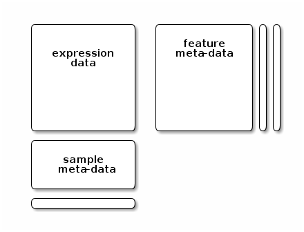
An assay data slot containing the quantitative omics data (expression data), stored as a
matrix. Features (genes, transcripts, proteins, …) are defined along the rows and samples along the columns.A sample metadata slot containing sample co-variates, stored as a table (
data.frameorDataFrame). This dataframe is stored with rows representing samples and sample covariate along the columns, and its rows match the expression data columns exactly.A feature metadata slot containing feature co-variates, stored as table annotated (
data.frameorDataFrame). This dataframe’s rows match the expression data rows exactly.
The coordinated nature of the high throughput data guarantees that the dimensions of the different slots will always match (i.e the columns in the expression data and then rows in the sample metadata, as well as the rows in the expression data and feature metadata) during data manipulation. The metadata slots can grow additional co-variates (columns) without affecting the other structures.
To illustrate such an omics data container, we’ll use a variable of
class SummarizedExperiment. Below, we load the GSE96870_intro
dataset from the rWSBIM1207 package (version >= 0.1.15).
## [1] "RangedSummarizedExperiment"
## attr(,"package")
## [1] "SummarizedExperiment"## class: RangedSummarizedExperiment
## dim: 1474 22
## metadata(0):
## assays(1): counts
## rownames(1474): Asl Apod ... Pbx1 Rgs4
## rowData names(11): gene ENTREZID ... phenotype_description
## hsapiens_homolog_associated_gene_name
## colnames(22): GSM2545336 GSM2545337 ... GSM2545363 GSM2545380
## colData names(10): title geo_accession ... tissue mouseThis data contains the same RNA-sequencing data as we have seen in
chapter 4. It is however formatted as a special
type of data, a SummarizedExperiment, that is specialised for
quantitative omics data (as opposed to the more general data.frame
data structure). We will be learning and using SummarizedExperiment
objects a lot in the
WSBIM1322 and
WSBIM2122 courses.
The object contains data for 1474 features (transcripts in this case) and 22 samples.
## [1] 1474 22## [1] 1474## [1] 22The samples (columns) and rows (protein features) are named:
##  [1] "GSM2545336" "GSM2545337" "GSM2545338" "GSM2545339" "GSM2545340"
##  [6] "GSM2545341" "GSM2545342" "GSM2545343" "GSM2545344" "GSM2545345"
## [11] "GSM2545346" "GSM2545347" "GSM2545348" "GSM2545349" "GSM2545350"
## [16] "GSM2545351" "GSM2545352" "GSM2545353" "GSM2545354" "GSM2545362"
## [21] "GSM2545363" "GSM2545380"## [1] "Asl" "Apod" "Cyp2d22" "Klk6" "Fcrls" "Slc2a4"## [1] "Mgst3" "Lrrc52" "Rxrg" "Lmx1a" "Pbx1" "Rgs4"Using this data structure, we can access the expression matrix with
the assay function, the feature metadata with the rowData function,
and the sample metadata with the colData function:
##         GSM2545336 GSM2545337 GSM2545338 GSM2545339 GSM2545340 GSM2545341
## Asl           1170        361        400        586        626        988
## Apod         36194      10347       9173      10620      13021      29594
## Cyp2d22       4060       1616       1603       1901       2171       3349
## Klk6           287        629        641        578        448        195
##         GSM2545342 GSM2545343 GSM2545344 GSM2545345 GSM2545346 GSM2545347
## Asl            836        535        586        597        938       1035
## Apod         24959      13668      13230      15868      27769      34301
## Cyp2d22       3122       2008       2254       2277       2985       3452
## Klk6           186       1101        537        567        327        233
##         GSM2545348 GSM2545349 GSM2545350 GSM2545351 GSM2545352 GSM2545353
## Asl            494        481        666        937        803        541
## Apod         11258      11812      15816      29242      20415      13682
## Cyp2d22       1883       2014       2417       3678       2920       2216
## Klk6           742        881        828        250        798        710
##         GSM2545354 GSM2545362 GSM2545363 GSM2545380
## Asl            473        748        576       1192
## Apod         11088      15916      11166      38148
## Cyp2d22       1821       2842       2011       4019
## Klk6           894        501        598        259
## [ reached 'max' / getOption("max.print") -- omitted 2 rows ]## DataFrame with 6 rows and 11 columns
## gene ENTREZID product gbkey
## <character> <character> <character> <character>
## Asl Asl 109900 argininosuccinate ly.. mRNA
## Apod Apod 11815 apolipoprotein D, tr.. mRNA
## Cyp2d22 Cyp2d22 56448 cytochrome P450, fam.. mRNA
## Klk6 Klk6 19144 kallikrein related-p.. mRNA
## Fcrls Fcrls 80891 Fc receptor-like S, .. mRNA
## Slc2a4 Slc2a4 20528 solute carrier famil.. mRNA
## external_gene_name ensembl_gene_id external_synonym chromosome_name
## <character> <character> <character> <character>
## Asl Asl ENSMUSG00000025533 2510006M18Rik 5
## Apod Apod ENSMUSG00000022548 NA 16
## Cyp2d22 Cyp2d22 ENSMUSG00000061740 2D22 15
## Klk6 Klk6 ENSMUSG00000050063 Bssp 7
## Fcrls Fcrls ENSMUSG00000015852 2810439C17Rik 3
## Slc2a4 Slc2a4 ENSMUSG00000018566 Glut-4 11
## gene_biotype phenotype_description
## <character> <character>
## Asl protein_coding abnormal circulating..
## Apod protein_coding abnormal lipid homeo..
## Cyp2d22 protein_coding abnormal skin morpho..
## Klk6 protein_coding abnormal cytokine le..
## Fcrls protein_coding decreased CD8-positi..
## Slc2a4 protein_coding abnormal circulating..
## hsapiens_homolog_associated_gene_name
## <character>
## Asl ASL
## Apod APOD
## Cyp2d22 CYP2D6
## Klk6 KLK6
## Fcrls FCRL4
## Slc2a4 SLC2A4## DataFrame with 22 rows and 10 columns
## title geo_accession organism age sex
## <character> <character> <character> <character> <factor>
## GSM2545336 CNS_RNA-seq_10C GSM2545336 Mus musculus 8 weeks Female
## GSM2545337 CNS_RNA-seq_11C GSM2545337 Mus musculus 8 weeks Female
## GSM2545338 CNS_RNA-seq_12C GSM2545338 Mus musculus 8 weeks Female
## GSM2545339 CNS_RNA-seq_13C GSM2545339 Mus musculus 8 weeks Female
## GSM2545340 CNS_RNA-seq_14C GSM2545340 Mus musculus 8 weeks Male
## ... ... ... ... ... ...
## GSM2545353 CNS_RNA-seq_3C GSM2545353 Mus musculus 8 weeks Female
## GSM2545354 CNS_RNA-seq_4C GSM2545354 Mus musculus 8 weeks Male
## GSM2545362 CNS_RNA-seq_5C GSM2545362 Mus musculus 8 weeks Female
## infection strain time tissue mouse
## <factor> <character> <factor> <factor> <factor>
## GSM2545336 InfluenzaA C57BL/6 Day8 Cerebellum 14
## GSM2545337 NonInfected C57BL/6 Day0 Cerebellum 9
## GSM2545338 NonInfected C57BL/6 Day0 Cerebellum 10
## GSM2545339 InfluenzaA C57BL/6 Day4 Cerebellum 15
## GSM2545340 InfluenzaA C57BL/6 Day4 Cerebellum 18
## ... ... ... ... ... ...
## GSM2545353 NonInfected C57BL/6 Day0 Cerebellum 4
## GSM2545354 NonInfected C57BL/6 Day0 Cerebellum 2
## GSM2545362 InfluenzaA C57BL/6 Day4 Cerebellum 20
## [ reached 'max' / getOption("max.print") -- omitted 2 rows ]► Question
Verify that the expression data dimensions match with number of rows and columns in the feature and sample data.
► Solution
We can use the [ operator to subset the whole object: all parts
thereof will be subset correctly.
## [1] 3 2## GSM2545337 GSM2545339
## Asl 361 586
## Cyp2d22 1616 1901
## Fcrls 233 237We can also add information with:
## DataFrame with 2 rows and 11 columns
##                      title geo_accession     organism         age      sex
##                <character>   <character>  <character> <character> <factor>
## GSM2545337 CNS_RNA-seq_11C    GSM2545337 Mus musculus     8 weeks   Female
## GSM2545339 CNS_RNA-seq_13C    GSM2545339 Mus musculus     8 weeks   Female
##              infection      strain     time     tissue    mouse     new_var
##               <factor> <character> <factor>   <factor> <factor> <character>
## GSM2545337 NonInfected     C57BL/6     Day0 Cerebellum       9     new_val1
## GSM2545339 InfluenzaA      C57BL/6     Day4 Cerebellum       15    new_val2
9.4.1 Saving objects
Exporting data to a spreadsheet using write.csv() or write_csv()
has several limitations, such as possible inconsistencies with , and
. for decimal separators and lack of variable type
definitions. Furthermore, exporting data to a spreadsheet is only
relevant for rectangular data such as data.frames and matrices and
isn’t applicable to more complex variables such as
SummarizedExperiment objects, that are themselves composed of
mulitple parts.
A more general way to save data, that is specific to R and is
guaranteed to work on any operating system, is to use the save()
function. Saving objects will generate a binary representation of the
object on disk, a R Data file (rda extension) that guarantees to
produce the same object once loaded back into R using the load()
function.
save(GSE96870_intro, file = "data_output/se.rda")
rm(GSE96870_intro)
load("data_output/se.rda")
GSE96870_intro
## class: RangedSummarizedExperiment
## dim: 1474 22
## metadata(0):
## assays(1): counts
## rownames(1474): Asl Apod ... Pbx1 Rgs4
## rowData names(11): gene ENTREZID ... phenotype_description
## hsapiens_homolog_associated_gene_name
## colnames(22): GSM2545336 GSM2545337 ... GSM2545363 GSM2545380
## colData names(10): title geo_accession ... tissue mouseNote how the load() function directly loads the object in the file
directly in the global environment using its original name.
The saveRDS() and readRDS() functions save R objects to binary
files (using the rds extension here) and read these back into
R. From a user’s perspective, the main difference is that, load()
loads an object in the global environment while readRDS() reads the
data from disk and returns it. It is thus necessary to store the
output of readRDS() in a variable:
## Loading required namespace: GenomeInfoDb## class: RangedSummarizedExperiment
## dim: 1474 22
## metadata(0):
## assays(1): counts
## rownames(1474): Asl Apod ... Pbx1 Rgs4
## rowData names(11): gene ENTREZID ... phenotype_description
## hsapiens_homolog_associated_gene_name
## colnames(22): GSM2545336 GSM2545337 ... GSM2545363 GSM2545380
## colData names(10): title geo_accession ... tissue mouseWhen it comes to saving data from R that will be loaded again in R, saving and loading is the preferred approach. If tabular data need to be shared with somebody who is not using R, then exporting to a text-based spreadsheet is a good alternative.
9.5 Bioconductor data infrastructure
An essential aspect that is central to Bioconductor and its success is the availability of core data infrastructure that is used across packages. Package developers are advised to make use of existing infrastructure to provide coherence, interoperability and stability to the project as a whole.
Here are some core classes, taken from the Common Bioconductor Methods and Classes page:
Importing
- GTF, GFF, BED, BigWig, etc., - rtracklayer
::import() - VCF – VariantAnnotation
::readVcf() - SAM / BAM – Rsamtools
::scanBam(), GenomicAlignments:readGAlignment*() - FASTA – Biostrings
::readDNAStringSet() - FASTQ – ShortRead
::readFastq() - Mass spectrometry data (XML-based and peaklist formats) – Spectra
::Spectra()
Common Classes
- Rectangular feature x sample data – SummarizedExperiment
::SummarizedExperiment()(RNAseq count matrix, microarray, proteomics, …) - Genomic coordinates – GenomicRanges
::GRanges()(1-based, closed interval) - DNA / RNA / AA sequences – Biostrings
::*StringSet() - Gene sets – GSEABase
::GeneSet()GSEABase::GeneSetCollection() - Multi-omics data – MultiAssayExperiment
::MultiAssayExperiment() - Single cell data – SingleCellExperiment
::SingleCellExperiment() - Mass spectrometry data – Spectra
::Spectra()
9.7 Exercises
► Question
Install a Bioconductor package of your choice, discover the vignette(s) it offers, open one, and extract the R code out of it.
Find a package that allows reading raw mass spectrometry data and identify the specific function. Either use the biocViews tree, look for a possible workflow, or look in the common methods and classes page on the Bioconductor page.
► Question
Load the
cptac_sedata from therWSBIM1322package. Verify it is of classSummarizedExperiment.Extract the quantitative information for the peptides
AIGVLPQLIIDR,NLDAAPTLRandYGLNHVVSLIENKKfor samples6A_7and6B_8. Subsetting works as we have seen fordata.framesin chapter 3.Look and interpret the experimental design stored in the sample metadata of this experiment. To help you out, you can also read its documentation.
What is the average expression of
LSAAQAELAYAETGAHDKin the groups6Aand6B?Calculate the average expression of all peptides belonging to protein
P02753ups|RETBP_HUMAN_UPSfor each sample. You can indentify which peptides to use by looking for that protein in the object’s rowData slot.
► Question
- To be able to access the data for this exercise, make sure you have
rWSBIM1207version 0.1.5 or later. If needed, install a more recent version with
Import the data from two tab-separated files into R. The full paths to the two files can be accessed with
kem.tsv(). Read?kemfor details on the content of the two files. In brief, thekem_counts.tsvfile contains RNA-Seq expression counts for 13 genes and 18 samples andkem_annot.tsvcontains annotation about each sample. Read the data into twotibblesnameskemandannotrespectively and familiarise yourself with the content of the two new tables.Convert the counts data into a long table format and annotate each sample using the experimental design.
Identify the three transcript identifiers that have the highest expression count over all samples.
Visualise the distribution of the expression for the three transcripts selected above in cell types A and B under both treatments.
For all genes, calculate the mean intensities in each experimental group (as defined by the
cell_typeandtreatmentvariables).Focusing only on the three most expressed transcripts and cell type A, calculate the fold-change induced by the treatment. The fold-change is the ratio between the average expressions in two conditions.
► Question
Download the following file and load its data. The
data is of class SummarizedExperiment and contains 9
genes for 27 samples.
Explore the object’s
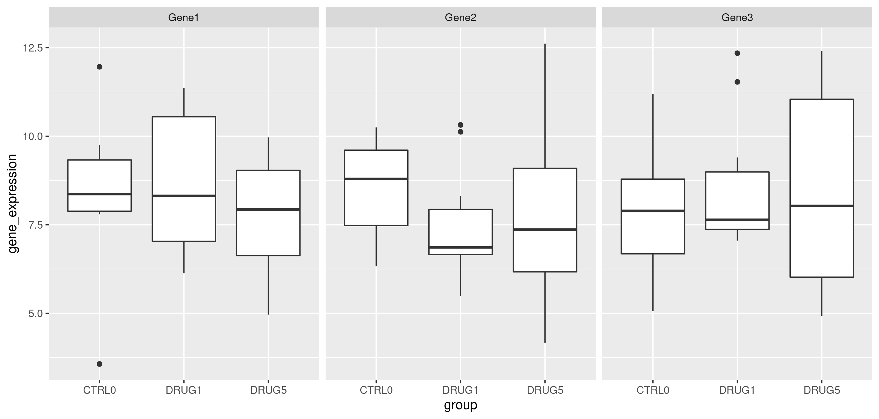
colDataand interprete it as the data’s experimental design.Generate a figure similar to the one below for your data own data.
Figure 9.7: Distribution of the gene expression in each group.
Calculate the average expression for each gene in each group.
Calculate the log2 fold-change (i.e. the difference of expression between two groups) for groups CTRL0 and DRUG5. Which gene shows the highest fold-change (i.e. where the expression increases most in DRUG5)? Can you recognise this on the figure?
Use the
var()function to calculate the variance for each gene. Which gene has the largest variance. Can you recognise this on the figure?Calculate the coefficient of variation of each gene. The coefficient of variation is defined as the ratio between a gene’s standard deviation (that you can compute using the
sd()function) and it’s mean. Which gene has the largest variance. Can you recognise this on the figure?Visualise the distribution of the gene expression in each sample. You can use either a boxplot, a violin plot or plot the density of these distributions with
geom_density(). Colour the sample data based on the groups.
Page built: 2026-04-02 using R version 4.5.0 (2025-04-11)