Chapter 8 Quantitative proteomics data analysis
Learning Objectives
The goals of this chapter are to provide a real-life example of step-by-step quantitative proteomics data analysis.
8.1 Introduction
Mass spectrometry-based quantitative proteomics data can be
representated as a matrix of quantitative values for features (PSMs,
peptides, proteins) arranged along the rows, measured for a set of
samples, arranged along the columns. The is a common representation
for any quantitative data set. As already done in
this
and
previous
course, we will be using the SummarizedExperiment class:
Figure 8.1: Schematic representation of the anatomy of a SummarizedExperiment object. (Figure taken from the SummarizedExperiment package vignette.)

- The sample (columns) metadata can be access with the
colData()function. - The features (rows) metadata can be access with the
rowData()column. - If the features represent ranges along genomic coordinates, these
can be accessed with
rowRanges() - Additional metadata describing the overall experiment can be
accessed with
metadata(). - The quantiative data can be accessed with
assay(). -
assays()returns a list of matrix-like assays.
8.2 QFeatures
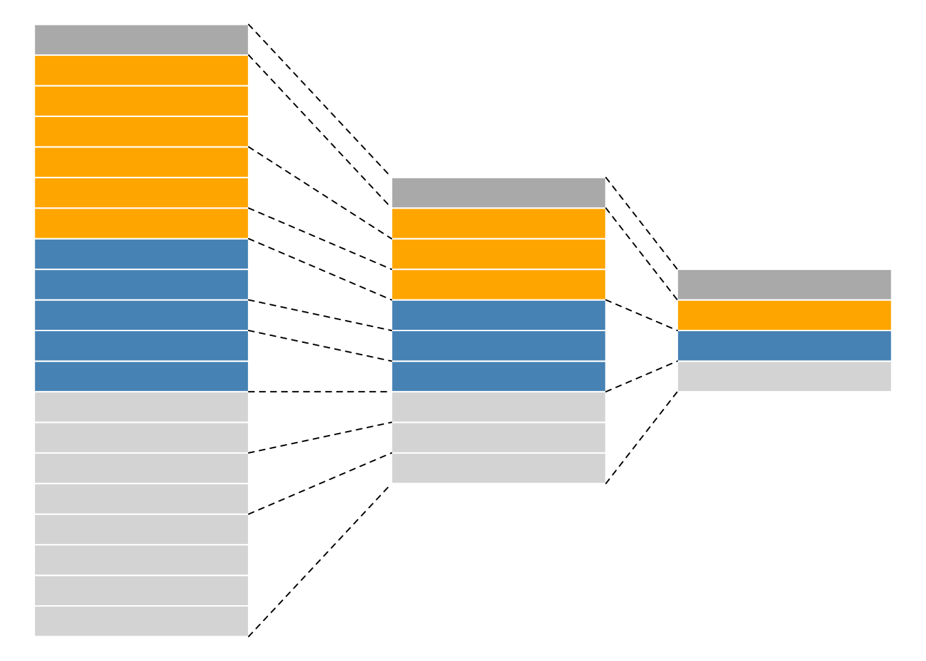
As we have already discussed in the previous chapter, even though mass spectrometers acquire data for spectra/peptides, the biological entities of interest remain the proteins. As part of the data processing, we are thus required to aggregate low-level quantitative features into higher level data.
Figure 8.2: Conceptual representation of a QFeatures object and the aggregative relation between different assays.
We are going to start to familiarise ourselves with the QFeatures
class implemented in the QFeatures
package. Let’s
start by loading the tidyverse and QFeatures packages.
 Figure 8.3: The
 QFeatures package.
Next, we load the feat1 test data, which is composed of single
assay of class SummarizedExperiment composed of 10 rows and 2
columns.
## An instance of class QFeatures (type: bulk) with 1 set:
##
##  [1] psms: SummarizedExperiment with 10 rows and 2 columns
► Question
Perform the following to familiarise yourselves with the QFeatures class:
Extract the sample metadata using the
colData()accessor (like you have previously done withSummarizedExperimentobjects).Extract the first (and only) assay composing this
QFeauresdata using the[[operator (as you have done to extract elements of a list) by using the assay’s index or name.Extract the
psmsassay’s row data and quantitative values.
► Solution
8.3 Feature aggregation
The central functionality of the QFeatures infrastructure is the
aggregation of features into higher-level features while retaining the
link between the different levels. This can be done with the
aggregateFeatures()
function.
The call below will
- operate on the
psmsassay of thefeat1objects; - aggregate the rows the assay following the grouping defined in the
peptidesrow data variables; - perform aggregation using the
colMeans()function; - create a new assay named
peptidesand add it to thefeat1object.
## Aggregated: 1/1## An instance of class QFeatures (type: bulk) with 2 sets:
##
## [1] psms: SummarizedExperiment with 10 rows and 2 columns
## [2] peptides: SummarizedExperiment with 3 rows and 2 columns► Question
- Convince yourself that you understand the effect of feature aggregation.
- Repeat the calculations manually.
- Observe the content of the new assay’s row data.
► Solution
► Question
Aggregate the peptide-level data into a new protein-level assay using
the colMedians() aggregation function.
► Solution
8.4 Subsetting and filtering
The link between the assays becomes apparent when we now subset the
assays for protein A as shown below or using the subsetByFeature()
function. This creates a new instance of class QFeatures containing
assays with the expression data for protein, its peptides and their
PSMs.
## An instance of class QFeatures (type: bulk) with 3 sets:
##
##  [1] psms: SummarizedExperiment with 6 rows and 2 columns
##  [2] peptides: SummarizedExperiment with 2 rows and 2 columns
##  [3] proteins: SummarizedExperiment with 1 rows and 2 columns
The filterFeatures() function can be used to filter rows the assays
composing a QFeatures object using the row data variables. We can
for example retain rows that have a pval < 0.05, which would only
keep rows in the psms assay because the pval is only relevant for
that assay.
## 'pval' found in 1 out of 3 assay(s).## No filter applied to the following assay(s) because one or more
## filtering variables are missing in the rowData: peptides, proteins. You
## can control whether to remove or keep the features using the 'keep'
## argument (see '?filterFeature').## An instance of class QFeatures (type: bulk) with 3 sets:
##
## [1] psms: SummarizedExperiment with 4 rows and 2 columns
## [2] peptides: SummarizedExperiment with 0 rows and 2 columns
## [3] proteins: SummarizedExperiment with 0 rows and 2 columnsOn the other hand, if we filter assay rows for those that localise to the mitochondrion, we retain the relevant protein, peptides and PSMs.
## 'location' found in 3 out of 3 assay(s).## An instance of class QFeatures (type: bulk) with 3 sets:
##
## [1] psms: SummarizedExperiment with 6 rows and 2 columns
## [2] peptides: SummarizedExperiment with 2 rows and 2 columns
## [3] proteins: SummarizedExperiment with 1 rows and 2 columns► Question
Filter rows that do not localise to the mitochondrion.
► Solution
You can refer to the Quantitative features for mass spectrometry
data
vignette and the QFeature manual
page
for more details about the class.
8.5 Analysis pipeline
Quantitative proteomics data processing is composed of the following steps:
- Data import
- Exploratory data analysis (PCA)
- Missing data management (filtering and/or imputation)
- Data cleaning
- Transformation and normalisation
- Aggregation
- Downstream analysis
8.6 The CPTAC data
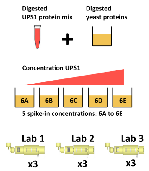
The CPTAC spike-in study 6 (Paulovich et al. 2010Paulovich, Amanda G, Dean Billheimer, Amy-Joan L Ham, Lorenzo Vega-Montoto, Paul A Rudnick, David L Tabb, Pei Wang, et al. 2010. “Interlaboratory Study Characterizing a Yeast Performance Standard for Benchmarking LC-MS Platform Performance.” Mol. Cell. Proteomics 9 (2): 242–54.) combines the Sigma UPS1 standard containing 48 different human proteins that are spiked in at 5 different concentrations (conditions A to E) into a constant yeast protein background. The sample were acquired in triplicate on different instruments in different labs. We are going to start with a subset of the CPTAC study 6 containing conditions A and B for a single lab.
Figure 8.4: The CPTAC spike-in study design (credit Lieven Clement, statOmics, Ghent University).
The peptide-level data, as processed by MaxQuant (Cox and Mann 2008Cox, J, and M Mann. 2008. “MaxQuant Enables High Peptide Identification Rates, Individualized p.p.b.-Range Mass Accuracies and Proteome-Wide Protein Quantification.” Nat Biotechnol 26 (12): 1367–72. https://doi.org/10.1038/nbt.1511.) is
available in the msdata package:
## [1] "cptac_a_b_peptides.txt"From the names of the columns, we see that the quantitative columns,
starting with "Intensity." (note the dot!) are at positions 56 to
61.
##  [1] "Sequence"                 "N.term.cleavage.window"
##  [3] "C.term.cleavage.window"   "Amino.acid.before"
##  [5] "First.amino.acid"         "Second.amino.acid"
##  [7] "Second.last.amino.acid"   "Last.amino.acid"
##  [9] "Amino.acid.after"         "A.Count"
## [11] "R.Count"                  "N.Count"
## [13] "D.Count"                  "C.Count"
## [15] "Q.Count"                  "E.Count"
## [17] "G.Count"                  "H.Count"
## [19] "I.Count"                  "L.Count"
## [21] "K.Count"                  "M.Count"
## [23] "F.Count"                  "P.Count"
## [25] "S.Count"                  "T.Count"
## [27] "W.Count"                  "Y.Count"
## [29] "V.Count"                  "U.Count"
## [31] "Length"                   "Missed.cleavages"
## [33] "Mass"                     "Proteins"
## [35] "Leading.razor.protein"    "Start.position"
## [37] "End.position"             "Unique..Groups."
## [39] "Unique..Proteins."        "Charges"
## [41] "PEP"                      "Score"
## [43] "Identification.type.6A_7" "Identification.type.6A_8"
## [45] "Identification.type.6A_9" "Identification.type.6B_7"
## [47] "Identification.type.6B_8" "Identification.type.6B_9"
## [49] "Experiment.6A_7"          "Experiment.6A_8"
## [51] "Experiment.6A_9"          "Experiment.6B_7"
## [53] "Experiment.6B_8"          "Experiment.6B_9"
## [55] "Intensity"                "Intensity.6A_7"
## [57] "Intensity.6A_8"           "Intensity.6A_9"
## [59] "Intensity.6B_7"           "Intensity.6B_8"
## [61] "Intensity.6B_9"           "Reverse"
## [63] "Potential.contaminant"    "id"
## [65] "Protein.group.IDs"        "Mod..peptide.IDs"
## [67] "Evidence.IDs"             "MS.MS.IDs"
## [69] "Best.MS.MS"               "Oxidation..M..site.IDs"
## [71] "MS.MS.Count"## [1] 56 57 58 59 60 61We now read these data using the readSummarizedExperiment
function. This peptide-level expression data will be imported into R
as an instance of class SummarizedExperiment. We also use the
fnames argument to set the row-names of the peptides assay to the
peptide sequences and specify that the file is a tab-separated table.
## class: SummarizedExperiment
## dim: 11466 6
## metadata(0):
## assays(1): ''
## rownames(11466): AAAAGAGGAGDSGDAVTK AAAALAGGK ... YYTVFDRDNNR
##   YYTVFDRDNNRVGFAEAAR
## rowData names(65): Sequence N.term.cleavage.window ...
##   Oxidation..M..site.IDs MS.MS.Count
## colnames(6): Intensity.6A_7 Intensity.6A_8 ... Intensity.6B_8
##   Intensity.6B_9
## colData names(0):
Before proceeding, we are going to clean up the sample names and annotate the experiment:
colnames(cptac_se) <- sub("I.+\\.", "", colnames(cptac_se))
cptac_se$condition <- sub("_[7-9]", "", colnames(cptac_se))
cptac_se$id <- sub("^.+_", "", colnames(cptac_se))
colData(cptac_se)
## DataFrame with 6 rows and 2 columns
## condition id
## <character> <character>
## 6A_7 6A 7
## 6A_8 6A 8
## 6A_9 6A 9
## 6B_7 6B 7
## 6B_8 6B 8
## 6B_9 6B 9Let’s also keep only a subset of
8.7 Missing values
Missing values can be highly frequent in proteomics. These exist two reasons supporting the existence of missing values, namely biological or technical.
Values that are missing due to the absence (or extremely low contentration) of a protein are observed for biological reasons, and their pattern aren’t random. A protein missing due to the suppression of its expression will not be missing at random: it will be missing in the condition in which it was suppressed, and be present in the condition where it is expressed.
Due to it’s data-dependent acquisition, mass spectrometry isn’t capable to assaying all peptides in a sample. Peptides that are less abundant than some of their co-eluting ions, peptides that do not ionise well or peptides that do not get identified might be sporadically missing in the final quantitation table, despite their presence in the biological samples. Their absence patterns are random in such cases.
Often, third party software that produce quantiative data use zeros
instead of properly reporting missing values. We can use the
zeroIsNA() function to replace the 0 by NA values in our
cptac_se object and then explore the missing data patterns across
columns and rows.
## $nNA
## DataFrame with 1 row and 2 columns
##         nNA       pNA
##   <integer> <numeric>
## 1     31130  0.452497
##
## $nNArows
## DataFrame with 11466 rows and 3 columns
##                name       nNA       pNA
##         <character> <integer> <numeric>
## 1     AAAAGAGGAG...         4  0.666667
## 2         AAAALAGGK         0  0.000000
## 3        AAAALAGGKK         0  0.000000
## 4     AAADALSDLE...         0  0.000000
## 5     AAADALSDLE...         0  0.000000
## ...             ...       ...       ...
## 11462 YYSIYDLGNN...         6  1.000000
## 11463 YYTFNGPNYN...         3  0.500000
## 11464    YYTITEVATR         4  0.666667
## 11465 YYTVFDRDNN...         6  1.000000
## 11466 YYTVFDRDNN...         6  1.000000
##
## $nNAcols
## DataFrame with 6 rows and 3 columns
##          name       nNA       pNA
##   <character> <integer> <numeric>
## 1        6A_7      4743  0.413658
## 2        6A_8      5483  0.478196
## 3        6A_9      5320  0.463980
## 4        6B_7      4721  0.411739
## 5        6B_8      5563  0.485174
## 6        6B_9      5300  0.462236
Figure 8.5: Distribution of missing value (white). Peptides row with more missing values are moved towards the top of the figure.
► Question
Explore the number or proportion of missing values across peptides and samples of the
cptac_sedata.Remove row that have too many missing values. You can do this by hand or using the
filterNA()function.
► Solution

8.8 Imputation
Imputation is the technique of replacing missing data with probable
values. This can be done with impute() method. As we have discussed
above, there are however two types of missing values in mass
spectrometry-based proteomics, namely data missing at random (MAR),
and data missing not at random (MNAR). These two types of missing data
need to be imputed with different types of imputation
methods
(Lazar et al. 2016Lazar, C, L Gatto, M Ferro, C Bruley, and T Burger. 2016. “Accounting for the Multiple Natures of Missing Values in Label-Free Quantitative Proteomics Data Sets to Compare Imputation Strategies.” J Proteome Res 15 (4): 1116–25. https://doi.org/10.1021/acs.jproteome.5b00981.).
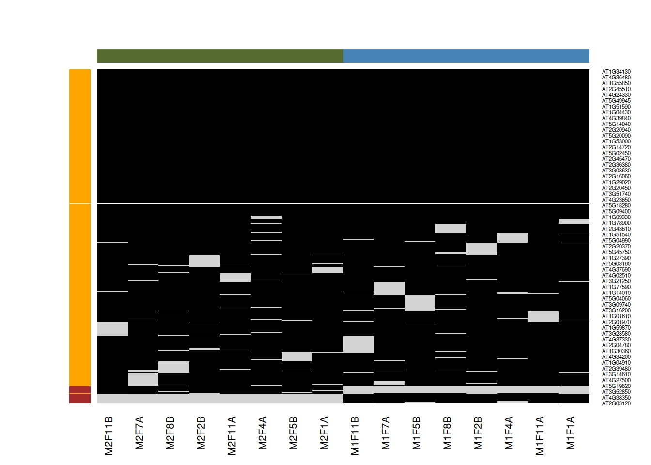
Figure 8.6: Mixed imputation method. Black cells represent presence of quantitation values and light grey corresponds to missing data. The two groups of interest are depicted in green and blue along the heatmap columns. Two classes of proteins are annotated on the left: yellow are proteins with randomly occurring missing values (if any) while proteins in brown are candidates for non-random missing value imputation.
When downstream analyses permit, it might thus be safer not to impute data and deal explicitly with missing values. This is possible when performing hypothesis tests, but not to perform a principal component analysis.
8.9 Identification quality control
As discussed in the previous chapter, PSMs are deemed relevant after
comparison against hist from a decoy database. The origin of these
hits is recorded with + in the Reverse variable:
##
##         +
## 7572   12
Similarly, a proteomics experiment is also searched against a database of contaminants:
##
## +
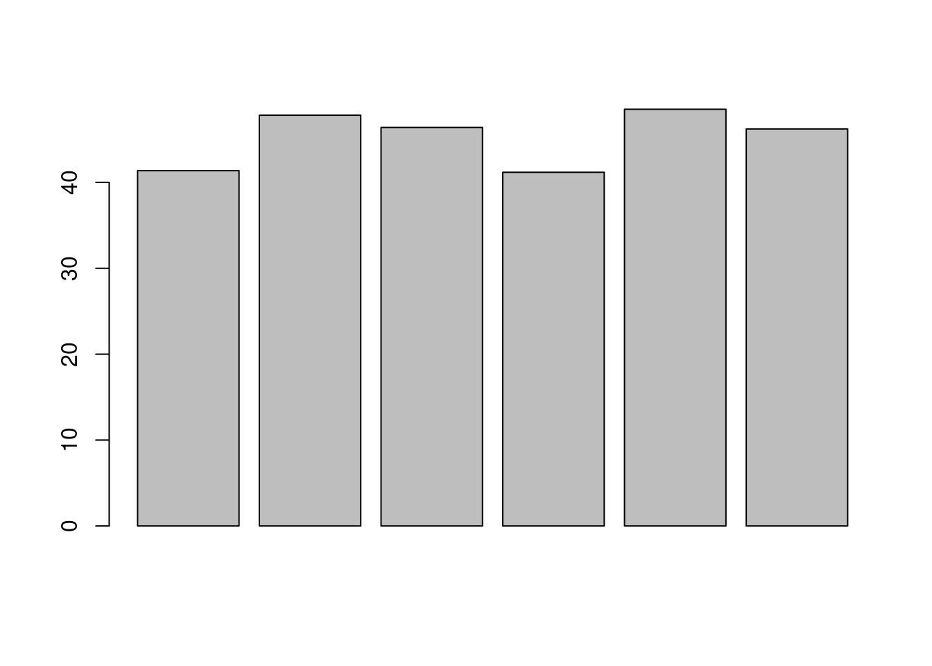
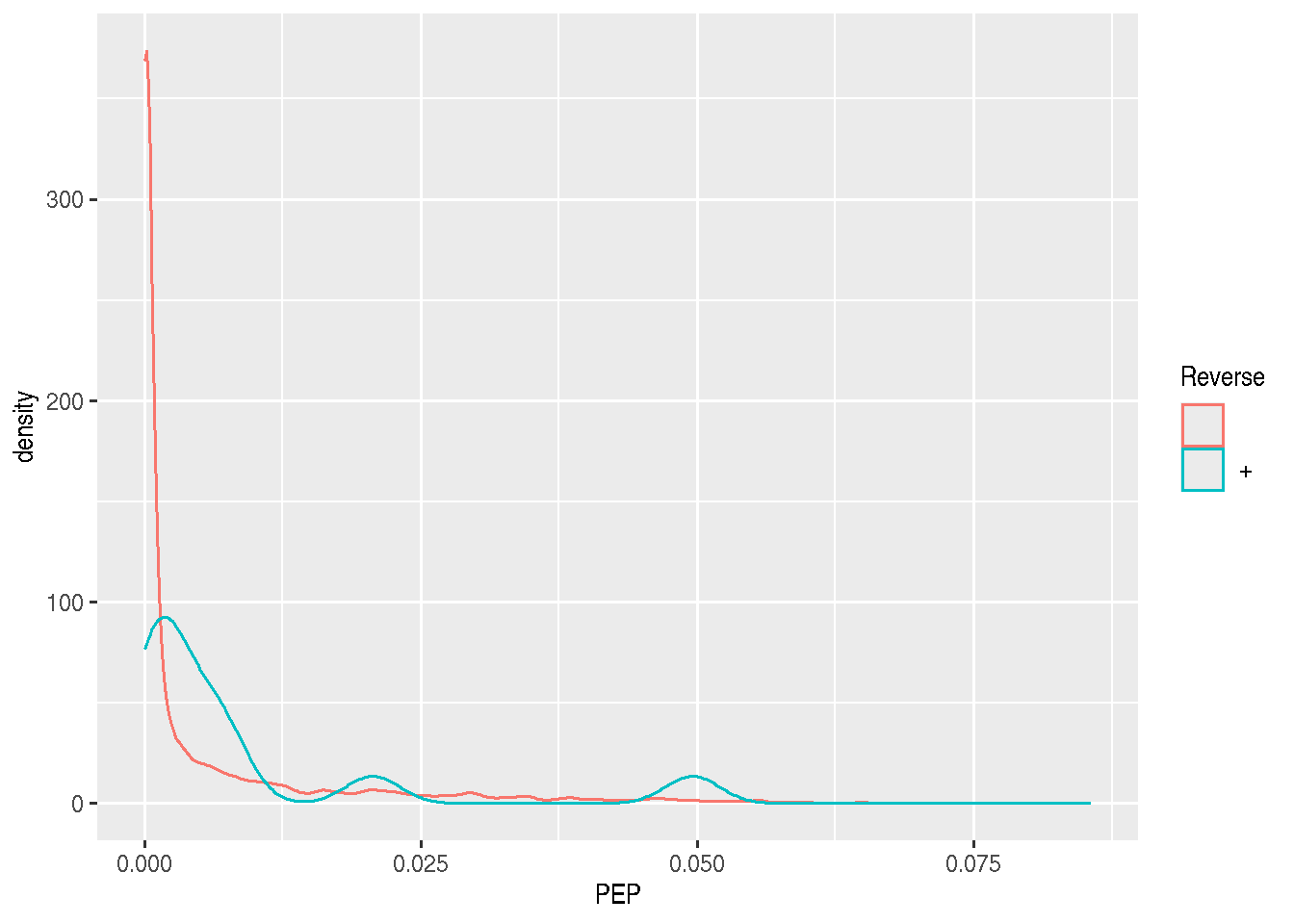
## 7558 26► Question
Visualise the score distributions from forward and reverse hits and interpret the figure.
Do the same with the posterior probability score (PEP).
► Solution
8.10 Creating the QFeatures data
We can now create our QFeatures object using the
SummarizedExperiment as show below.
We should also assign the QFeatures column data with the
SummarizedExperiment slot.
Note that it is also possible to directly create a QFeatures object
with the readQFeatures() function and the same arguments as the
readSummarizedExperiment() used above. In addition, most functions
used above and below work on single SummarizedExperiment objects or
assays within a QFeatures object.
8.11 Filtering out contaminants and reverse hits
► Question
Using the filterFeatures() function, filter out the reverse and
contaminant hits.
► Solution
8.12 Log-transformation and normalisation
The two code chunks below log-transform and normalise using the assay
i as input and adding a new one names as defined by name.
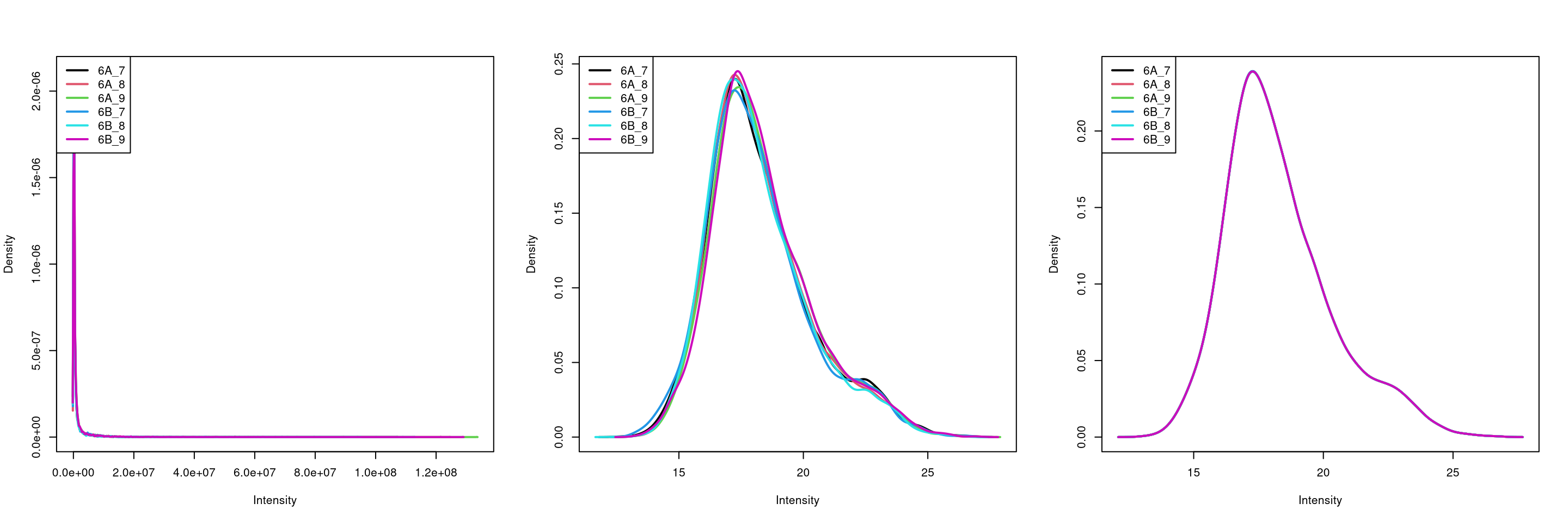
par(mfrow = c(1, 3))
limma::plotDensities(assay(cptac[["peptides"]]))
limma::plotDensities(assay(cptac[["log_peptides"]]))
limma::plotDensities(assay(cptac[["lognorm_peptides"]]))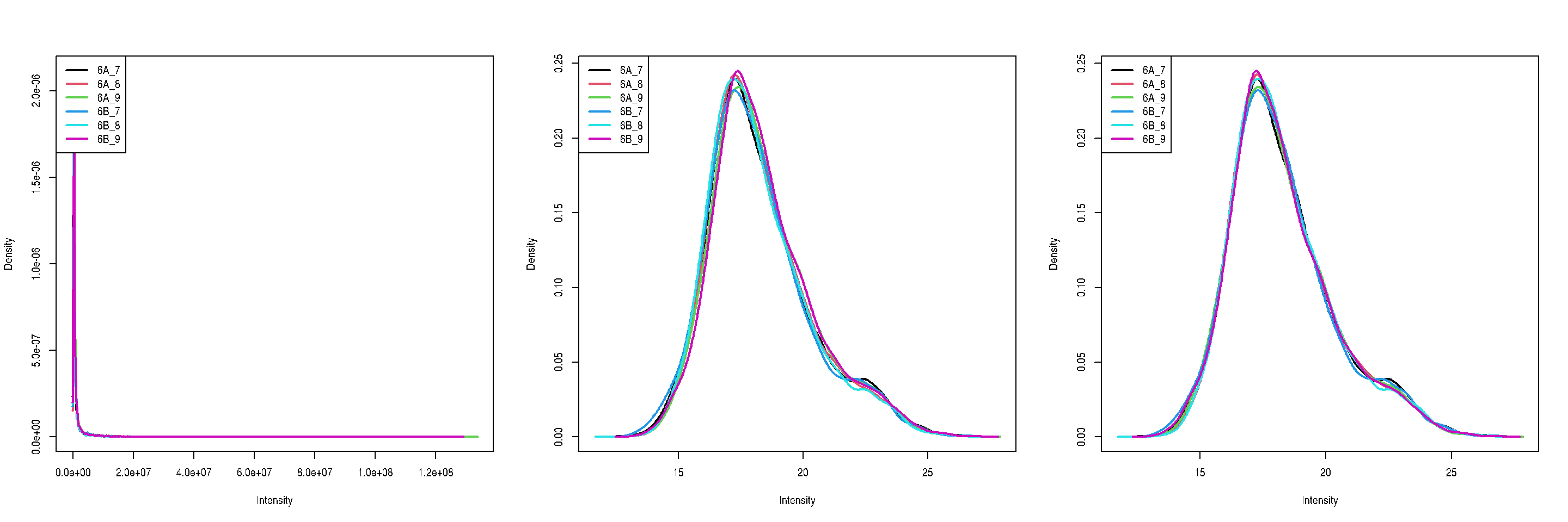
Figure 8.7: Three peptide level assays: raw data, log transformed and normalised.
8.13 Aggregation
Below, we are going to use median aggregation, as a first attempt. This is however not the best choice, as we will see later.
cptac <-
    aggregateFeatures(cptac,
                      "lognorm_peptides",
                      name = "proteins_med",
                      fcol = "Leading.razor.protein",
                      fun = colMedians,
                      na.rm = TRUE)
Looking at the .n row variable computed during the aggregation, we
see that most proteins result of the aggregation of 5 peptides or
less, while very few proteins are accounted for by tens of peptides.
##
##   1   2   3   4   5   6   7   8   9  10  11  12  13  14  15  16  17  18  19  20
## 328 234 162 138  85  72  66  49  46  34  25  28  21  12  17   9   5   4  13   5
##  21  22  23  24  25  26  28  29  30  31  32  35  38  39  42  43  51  52  62
##   7   6   4   4   3   3   1   3   1   1   3   1   2   1   1   1   1   1   1
8.14 Principal component analysis
library("factoextra")
library("patchwork")

pca_pep <-
    cptac[["lognorm_peptides"]] %>%
    filterNA() %>%
    assay() %>%
    t() %>%
    prcomp(scale = TRUE, center = TRUE) %>%
    fviz_pca_ind(habillage = cptac$condition, title = "Peptides")

pca_prot <-
    cptac[["proteins_med"]] %>%
    filterNA() %>%
    assay() %>%
    t() %>%
    prcomp(scale = TRUE, center = TRUE) %>%
    fviz_pca_ind(habillage = cptac$condition,
                 title = "Proteins (median aggregation)")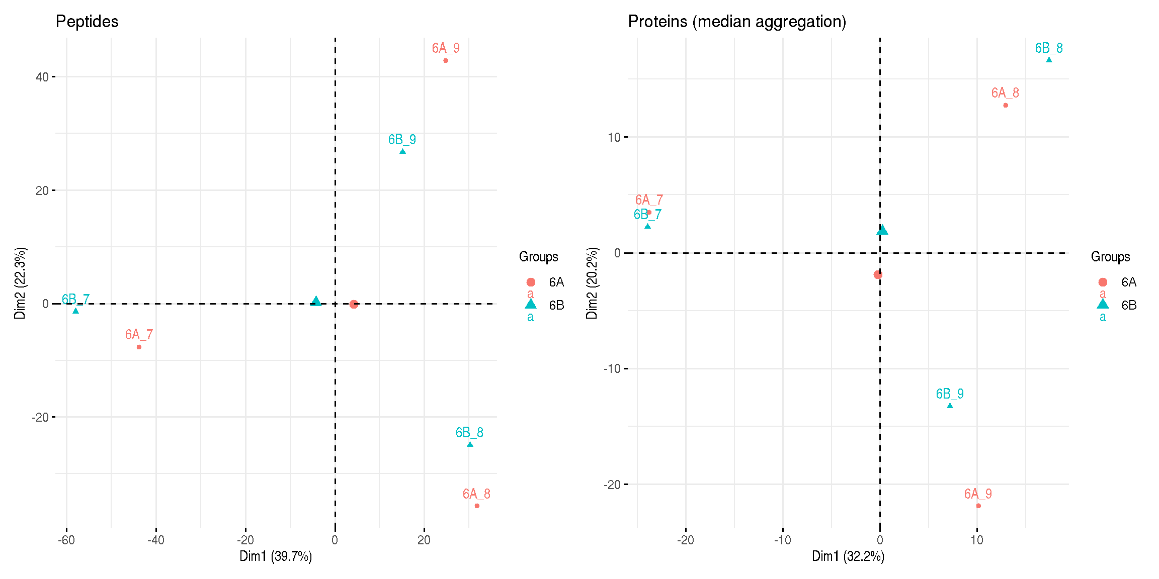
Figure 8.8: Peptide and protein level PCA analyses.
► Question
Interpret the two PCA plots above.
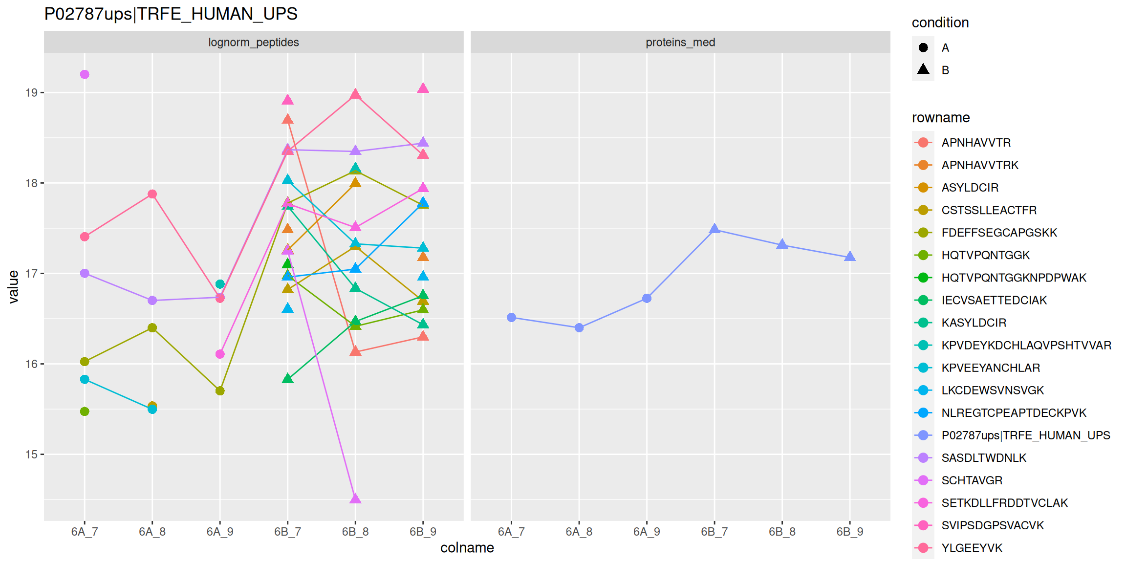
8.15 Visualisation
Below, we use the longForm() function to extract the quantitative
and row data in a long format, that can be directly reused by the
tidyverse tools.
longForm(cptac["P02787ups|TRFE_HUMAN_UPS", ,
               c("lognorm_peptides", "proteins_med")]) %>%
    as_tibble() %>%
    mutate(condition = ifelse(grepl("A", colname), "A", "B")) %>%
    ggplot(aes(x = colname, y = value, colour = rowname, shape = condition)) +
    geom_point(size = 3) +
    geom_line(aes(group = rowname)) +
    facet_grid(~ assay) +
    ggtitle("P02787ups|TRFE_HUMAN_UPS")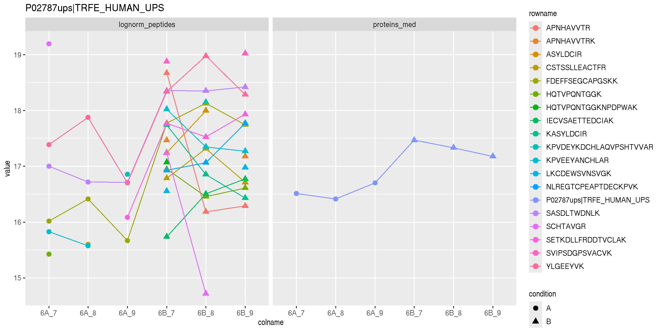
Figure 8.9: Peptide and protein expression profile.
8.16 Statistical analysis
Below, we are going to perform our statistical analysis on the protein data.
We have seen in chapter 2 how to use linear models and have applied the same prinicples in chapter 4 on count data (based on a negative binomial distribution). The limma package is the precursor package that enables the consistent application of linear models to normally distributed omics data in general, and microarrays in particuar15 The name of the package refers to Linear Models for Microarray Data..
The limma package also implements an empirical Bayes method that
borrows information across features to estimate the standard
error16 alike the shinkage gene-wise dispersion estimates see in
DESeq2. and calculate (so called moderate) t
statistics. This approach is demonstrably more powerful than a
standard t-tests when the number of samples is lot.
The code chunk below illstrated how to set up the model, fit it, and apply the empirical Bayes moderation.
## Warning: Partial NA coefficients for 23 probe(s)Finally, the topTable() function is used the extract the results for
the coefficient of interest. You can look at the column names of the
coefficients table to get their names.
## [1] "(Intercept)" "prots$condition6B"res <-
topTable(fit, coef = "prots$condition6B", number = Inf) %>%
rownames_to_column("protein") %>%
as_tibble() %>%
mutate(TP = grepl("ups", protein))► Question
Note the warning about partial NA coefficients for 23 probes. Where
could these come from?
► Solution
vp <-
    res %>%
    ggplot(aes(x = logFC, y = -log10(adj.P.Val))) +
    geom_point(aes(colour = TP)) +
    geom_vline(xintercept = c(-1, 1)) +
    geom_hline(yintercept = -log10(0.05)) +
scale_color_manual(values = c("black","red"))Using the pipeline described above, we would would identify a single differentially expressed protein at an 5 percent FDR but miss out the other 32 expected spike-in proteins. We can assess our results in terms of true/false postitves/negatives:
- True positives: 1
- False positives: 0
- True negatives: 1342
- False negatives: 32
As shown below, it is possible to substantially improve these results using robust summarisation, i.e robust regression with M-estimation using Huber weights, as described in section 2.7 in (Sticker et al. 2019Sticker, Adriaan, Ludger Goeminne, Lennart Martens, and Lieven Clement. 2019. “Robust Summarization and Inference in Proteome-Wide Label-Free Quantification.” bioRxiv. https://doi.org/10.1101/668863.).
Figure 8.10: Aggregation using robust summarisation.
- True positives: 21
- False positives: 2
- True negatives: 1340
- False negatives: 12
8.17 Project
You are provided with the larger CPTAC data including a third condition (namely C) and a two additional lab, tallying now 27 samples.
| LTQ-Orbitrap_86 | LTQ-OrbitrapO_65 | LTQ-OrbitrapW_56 | |
|---|---|---|---|
| 6A | 3 | 3 | 3 |
| 6B | 3 | 3 | 3 |
| 6C | 3 | 3 | 3 |
The full design is shown below and is available here.
| TRUE | id | condition | lab | previous |
|---|---|---|---|---|
| 6A_1 | 1 | 6A | LTQ-Orbitrap_86 | new |
| 6A_2 | 2 | 6A | LTQ-Orbitrap_86 | new |
| 6A_3 | 3 | 6A | LTQ-Orbitrap_86 | new |
| 6A_4 | 4 | 6A | LTQ-OrbitrapO_65 | new |
| 6A_5 | 5 | 6A | LTQ-OrbitrapO_65 | new |
| 6A_6 | 6 | 6A | LTQ-OrbitrapO_65 | new |
| 6A_7 | 7 | 6A | LTQ-OrbitrapW_56 | |
| 6A_8 | 8 | 6A | LTQ-OrbitrapW_56 | |
| 6A_9 | 9 | 6A | LTQ-OrbitrapW_56 | |
| 6B_1 | 1 | 6B | LTQ-Orbitrap_86 | new |
| 6B_2 | 2 | 6B | LTQ-Orbitrap_86 | new |
| 6B_3 | 3 | 6B | LTQ-Orbitrap_86 | new |
| 6B_4 | 4 | 6B | LTQ-OrbitrapO_65 | new |
| 6B_5 | 5 | 6B | LTQ-OrbitrapO_65 | new |
| 6B_6 | 6 | 6B | LTQ-OrbitrapO_65 | new |
| 6B_7 | 7 | 6B | LTQ-OrbitrapW_56 | |
| 6B_8 | 8 | 6B | LTQ-OrbitrapW_56 | |
| 6B_9 | 9 | 6B | LTQ-OrbitrapW_56 | |
| 6C_1 | 1 | 6C | LTQ-Orbitrap_86 | new |
| 6C_2 | 2 | 6C | LTQ-Orbitrap_86 | new |
| 6C_3 | 3 | 6C | LTQ-Orbitrap_86 | new |
| 6C_4 | 4 | 6C | LTQ-OrbitrapO_65 | new |
| 6C_5 | 5 | 6C | LTQ-OrbitrapO_65 | new |
| 6C_6 | 6 | 6C | LTQ-OrbitrapO_65 | new |
| 6C_7 | 7 | 6C | LTQ-OrbitrapW_56 | new |
| 6C_8 | 8 | 6C | LTQ-OrbitrapW_56 | new |
| 6C_9 | 9 | 6C | LTQ-OrbitrapW_56 | new |
Page built: 2025-12-19 using R version 4.5.0 (2025-04-11)