CytoPipelineGUI : visualization of Flow Cytometry Data Analysis Pipelines run with CytoPipeline

Abstract

This vignette gives a short introduction to CytoPipelineGUI, which is the companion package of CytoPipeline for interactive visualization of flow cytometry data pre-processing pipeline results. This vignette is distributed under a CC BY-SA license.

Installation

To install this package, start R and enter (uncommented):

# if (!require("BiocManager", quietly = TRUE))
#     install.packages("BiocManager")
# 
# BiocManager::install("CytoPipelineGUI")

Foreword - Preparation of pipeline results to be visualized

CytoPipelineGUI is the companion package of CytoPipeline, and is used for interactive visualization of flow cytometry data pre-processing pipeline results. It implements two shiny applications :

a shiny app for interactive comparison of flow frames that are the results of CytoProcessingSteps of the same or different CytoPipeline experiments.
It is launched using the following statement: CytoPipelineCheckApp() (see below);
a shiny app for interactive visualization and manual adjustments of scale transformation objects. It is launched using the following statement: ScaleTransformApp() (see below).

In order to be able to show CytoPipelineGUI in action, as a pre-requisite we need to have created a CytoPipeline object, defined the different pipeline steps, and run the pipeline until completion, so that all intermediate results can be found on a cache. These preliminary steps are performed by the preparation code below.

# raw data
rawDataDir <- system.file("extdata", package = "CytoPipeline")
sampleFiles <- file.path(rawDataDir, list.files(rawDataDir,
                                                pattern = "Donor"))
# output files
workDir <- suppressMessages(base::tempdir())
# pipeline configuration files (in json)
jsonDir <- rawDataDir

# creation of CytoPipeline objects

pipL_PeacoQC <-
  CytoPipeline(file.path(jsonDir, "OMIP021_PeacoQC_pipeline.json"),
               experimentName = "OMIP021_PeacoQC",
               sampleFiles = sampleFiles)

pipL_flowAI <-
  CytoPipeline(file.path(jsonDir, "OMIP021_flowAI_pipeline.json"),
               experimentName = "OMIP021_flowAI",
               sampleFiles = sampleFiles)

# execute PeacoQC pipeline
suppressWarnings(execute(pipL_PeacoQC, rmCache = TRUE, path = workDir))

# execute flowAI pipeline
suppressWarnings(execute(pipL_flowAI, rmCache = TRUE, path = workDir))

## Quality control for the file: Donor1
## 5.46% of anomalous cells detected in the flow rate check. 
## 0% of anomalous cells detected in signal acquisition check. 
## 0.12% of anomalous cells detected in the dynamic range check.

## Quality control for the file: Donor2
## 66.42% of anomalous cells detected in the flow rate check. 
## 0% of anomalous cells detected in signal acquisition check. 
## 0.1% of anomalous cells detected in the dynamic range check.

If you are unfamiliar with CytoPipeline package, and you would like to know more about these steps, it is advised that you read the CytoPipeline vignette, and/or that you watch the videos illustrating the CytoPipeline suite, which are accessible through links included in the Demo.Rmd vignette.

Introduction

The visualization tools shown here are demonstrated on the results of two different previously run CytoPipeline objects. These flow cytometry pre-processing pipeline are described in details in the CytoPipeline vignette. Here below is a short summary of the illustrating dataset, as well as the pipeline steps.

Example dataset (more details in CytoPipeline vignette)

The example dataset that will be used throughout this vignette is derived from a reference public dataset accompanying the OMIP-021 (Optimized Multicolor Immunofluorescence Panel 021) article (Gherardin et al. 2014).

A sub-sample of this public dataset is built-in in the CytoPipeline package, as the OMIP021 dataset. See the MakeOMIP021Samples.R script for more details on how the OMIP021 dataset was created. This script is to be found in the script subdirectory in the CytoPipeline package installation path.

Example of pre-processing and QC pipelines (more details in CytoPipeline vignette)

In our example pipeline, we assumed that we wanted to pre-process the two samples of the OMIP021 dataset, and that we wanted to compare what we would obtain when pre-processing these files using two different QC methods.

In the first pre-processing pipeline, we used the flowAI QC method (Monaco et al. 2016), while in the second pipeline, we used the PeacoQC method (Emmaneel et al. 2021).

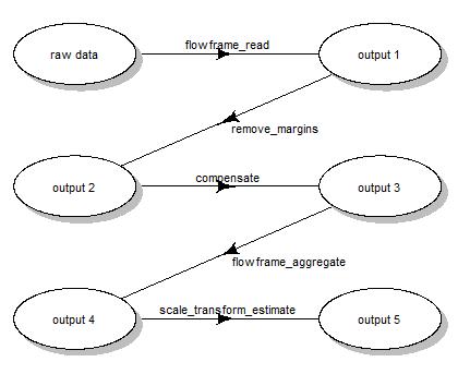
In both pipelines, the first part consisted in estimating appropriate scale transformation functions for all channels present in the sample flowFrame. For this, we ran the following steps (Fig. 1):

reading the two samples .fcs files
removing the margin events from each file
applying compensation for each file
aggregating and sub-sampling from each file
estimating the scale transformations from the aggregated and sub-sampled data

Scale transform processing queue

After this first part, pre-processing for each file, one by one, was performed.
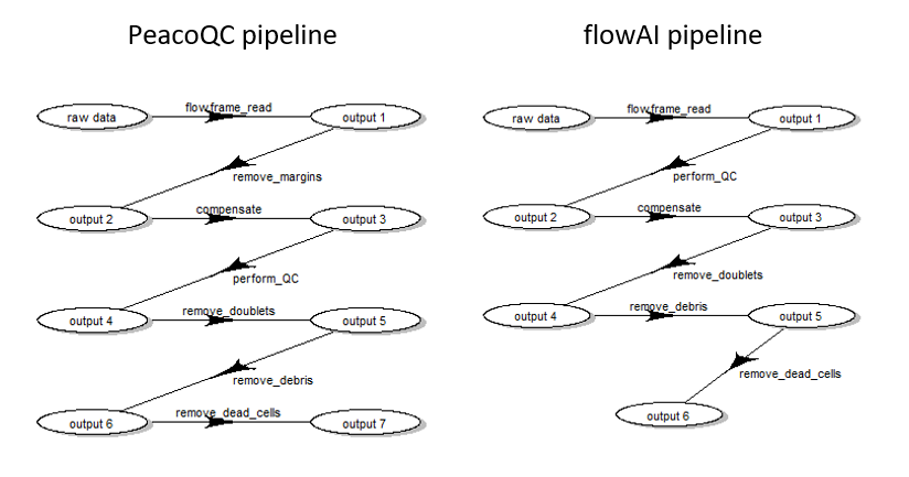
However, depending on the choice of QC method, the order of steps needed to be slightly different (see Fig. 2) :

Pre-processing queue for two different pipeline settings

Interactive visualizations

Visualizing pipeline runs at different steps

Using the CytoPipelineGUI package, it is possible to interactively inspect intermediate results produced during the pipeline execution.

This is done through the CytoPipelineCheckApp, which can provide a view of the data structure, i.e. the flowFrame, at any step of any pipeline, as well as a comparison between any the pair of flowFrame state.

if (interactive()) {
    CytoPipelineGUI::CytoPipelineCheckApp(dir = workDir)    
}

It is difficult to extensively demonstrate specific user interactions in a vignette, therefore live demo videos can be found from the Demo.Rmd vignette.

However, it is possible to mimic the call to some of the shiny application features, by using some specific CytoPipelineGUI exported functions.

A first example below is a function call which retrieves the visuals of the workflow of a previously run pipeline:

# pre-processing workflow
expName <- "OMIP021_PeacoQC"
CytoPipelineGUI::plotSelectedWorkflow(
            experimentName = expName,
            whichQueue = "pre-processing",
            sampleFile = sampleFiles[1],
            path = workDir)

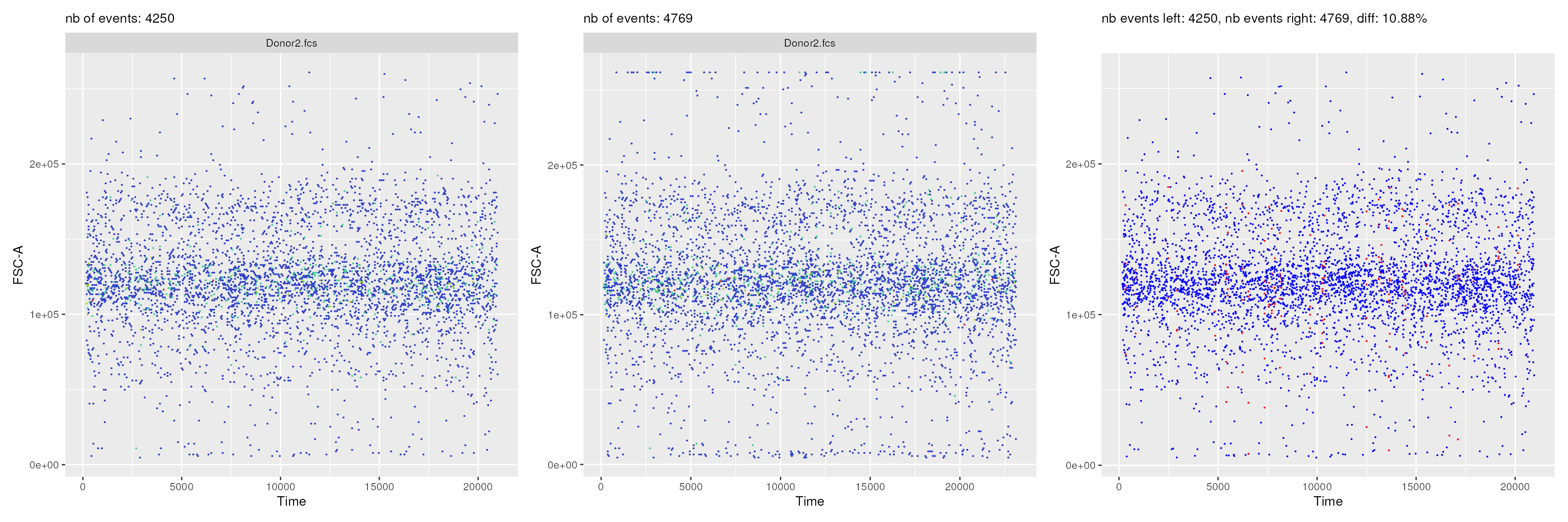
It is also possible to programmatically obtain comparison plots that are displayed within the shiny application.
Here below is an example, where one is comparing the two pipelines (PeacoQC vs flowAI) after the QC step:

expName1 <- "OMIP021_PeacoQC"
expName2 <- "OMIP021_flowAI"

p1 <- CytoPipelineGUI::plotSelectedFlowFrame(
    experimentName = expName1,
    whichQueue = "pre-processing",
    sampleFile = 2,
    flowFrameName = "perform_QC_obj",
    path = workDir,
    xChannelLabel = "Time : NA",
    yChannelLabel = "FSC-A : NA",
    useAllCells = TRUE,
    useFixedLinearRange = FALSE)

p2 <- CytoPipelineGUI::plotSelectedFlowFrame(
    experimentName = expName2,
    whichQueue = "pre-processing",
    sampleFile = 2, 
    flowFrameName = "perform_QC_obj",
    path = workDir,
    xChannelLabel = "Time : NA",
    yChannelLabel = "FSC-A : NA",
    useAllCells = TRUE,
    useFixedLinearRange = FALSE)

p3 <- CytoPipelineGUI::plotDiffFlowFrame(
    path = workDir,
    experimentNameFrom = expName1,
    whichQueueFrom = "pre-processing",
    sampleFileFrom = 2, 
    flowFrameNameFrom = "perform_QC_obj",
    xChannelLabelFrom = "Time : NA",
    yChannelLabelFrom = "FSC-A : NA",
    experimentNameTo = expName2,
    whichQueueTo = "pre-processing",
    sampleFileTo = 2,
    flowFrameNameTo = "perform_QC_obj",
    xChannelLabelTo = "Time : NA",
    yChannelLabelTo = "FSC-A : NA",
    useAllCells = TRUE,
    useFixedLinearRange = FALSE)

p1+p2+p3

Visualization of scale transformations

Besides the flowFrame comparison tool, CytoPipelineGUI provides another shiny app, which allows to interactively visualize and manage the scale transformations that are generated as part of our prep-processing pipelines.

If the shape of the scale transformations that were automatically set by the chosen algorithm appears to be non satisfactory, it is possible, using this shiny application, to manually adjust the parameters of the transformation, and save the results in a RDS object. This object can then be re-used in another pipeline instance.

# 5. show scale transformations
if (interactive()){
    CytoPipelineGUI::ScaleTransformApp(dir = workDir)    
}

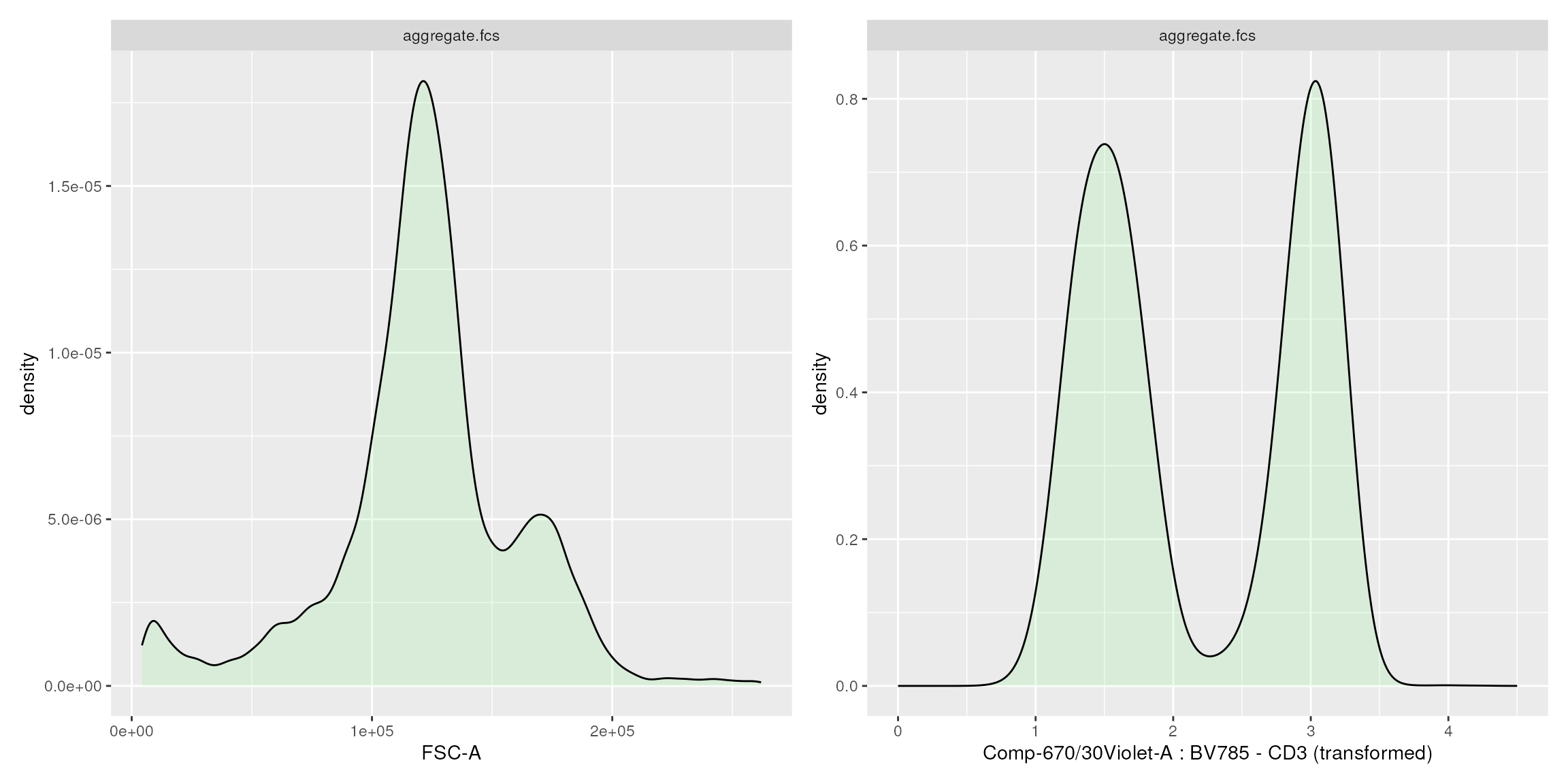
Note that here also, it is possible to obtain the visuals of the scale transformations programmatically, although this is a bit more evolved, as one has to use CytoPipeline functions for this.

expName <- "OMIP021_PeacoQC"
pipL <- CytoPipeline::buildCytoPipelineFromCache(
    experimentName = expName,
    path = workDir
)

    ff <- CytoPipeline::getCytoPipelineFlowFrame(
        pipL,
        path = workDir,
        whichQueue = "scale transform",
        objectName = "flowframe_aggregate_obj"
    )
    
    p1 <- plotScaleTransformedChannel(
        ff,
        channel = "FSC-A",
        transfoType = "linear",
        linA = 0.0002,
        linB = -0.5)
    
    p2 <- plotScaleTransformedChannel(
        ff,
        channel = "CD3",
        applyTransform = "data",
        transfoType = "logicle",
        negDecades = 1,
        width = 0.5,
        posDecades = 4
    )
    
    p1+p2

Session information

## R version 4.4.1 (2024-06-14)
## Platform: x86_64-pc-linux-gnu
## Running under: Ubuntu 22.04.5 LTS
## 
## Matrix products: default
## BLAS:   /usr/lib/x86_64-linux-gnu/openblas-pthread/libblas.so.3 
## LAPACK: /usr/lib/x86_64-linux-gnu/openblas-pthread/libopenblasp-r0.3.20.so;  LAPACK version 3.10.0
## 
## locale:
##  [1] LC_CTYPE=en_US.UTF-8       LC_NUMERIC=C              
##  [3] LC_TIME=en_US.UTF-8        LC_COLLATE=en_US.UTF-8    
##  [5] LC_MONETARY=en_US.UTF-8    LC_MESSAGES=en_US.UTF-8   
##  [7] LC_PAPER=en_US.UTF-8       LC_NAME=C                 
##  [9] LC_ADDRESS=C               LC_TELEPHONE=C            
## [11] LC_MEASUREMENT=en_US.UTF-8 LC_IDENTIFICATION=C       
## 
## time zone: UTC
## tzcode source: system (glibc)
## 
## attached base packages:
## [1] stats     graphics  grDevices utils     datasets  methods   base     
## 
## other attached packages:
## [1] patchwork_1.3.0       CytoPipelineGUI_1.5.1 CytoPipeline_1.6.0   
## [4] BiocStyle_2.34.0     
## 
## loaded via a namespace (and not attached):
##   [1] DBI_1.2.3             gridExtra_2.3         rlang_1.1.4          
##   [4] magrittr_2.0.3        clue_0.3-65           GetoptLong_1.0.5     
##   [7] matrixStats_1.4.1     compiler_4.4.1        RSQLite_2.3.7        
##  [10] png_0.1-8             systemfonts_1.1.0     vctrs_0.6.5          
##  [13] reshape2_1.4.4        stringr_1.5.1         pkgconfig_2.0.3      
##  [16] shape_1.4.6.1         crayon_1.5.3          fastmap_1.2.0        
##  [19] dbplyr_2.5.0          labeling_0.4.3        utf8_1.2.4           
##  [22] promises_1.3.0        ncdfFlow_2.52.0       rmarkdown_2.28       
##  [25] graph_1.84.0          ragg_1.3.3            purrr_1.0.2          
##  [28] bit_4.5.0             xfun_0.48             zlibbioc_1.52.0      
##  [31] cachem_1.1.0          jsonlite_1.8.9        flowWorkspace_4.18.0 
##  [34] blob_1.2.4            highr_0.11            later_1.3.2          
##  [37] parallel_4.4.1        cluster_2.1.6         R6_2.5.1             
##  [40] bslib_0.8.0           stringi_1.8.4         RColorBrewer_1.1-3   
##  [43] jquerylib_0.1.4       Rcpp_1.0.13           bookdown_0.41        
##  [46] iterators_1.0.14      knitr_1.48            zoo_1.8-12           
##  [49] IRanges_2.40.0        flowCore_2.18.0       httpuv_1.6.15        
##  [52] tidyselect_1.2.1      yaml_2.3.10           doParallel_1.0.17    
##  [55] codetools_0.2-20      curl_5.2.3            lattice_0.22-6       
##  [58] tibble_3.2.1          plyr_1.8.9            Biobase_2.66.0       
##  [61] shiny_1.9.1           withr_3.0.2           evaluate_1.0.1       
##  [64] desc_1.4.3            BiocFileCache_2.14.0  circlize_0.4.16      
##  [67] pillar_1.9.0          BiocManager_1.30.25   filelock_1.0.3       
##  [70] foreach_1.5.2         flowAI_1.36.0         stats4_4.4.1         
##  [73] generics_0.1.3        diagram_1.6.5         S4Vectors_0.44.0     
##  [76] ggplot2_3.5.1         munsell_0.5.1         ggcyto_1.34.0        
##  [79] scales_1.3.0          xtable_1.8-4          PeacoQC_1.16.0       
##  [82] changepoint_2.2.4     glue_1.8.0            tools_4.4.1          
##  [85] hexbin_1.28.4         data.table_1.16.2     fs_1.6.4             
##  [88] XML_3.99-0.17         grid_4.4.1            RProtoBufLib_2.18.0  
##  [91] colorspace_2.1-1      cli_3.6.3             textshaping_0.4.0    
##  [94] fansi_1.0.6           cytolib_2.18.0        ComplexHeatmap_2.22.0
##  [97] dplyr_1.1.4           Rgraphviz_2.50.0      gtable_0.3.6         
## [100] sass_0.4.9            digest_0.6.37         BiocGenerics_0.52.0  
## [103] rjson_0.2.23          htmlwidgets_1.6.4     farver_2.1.2         
## [106] memoise_2.0.1         htmltools_0.5.8.1     pkgdown_2.1.1.9000   
## [109] lifecycle_1.0.4       httr_1.4.7            GlobalOptions_0.1.2  
## [112] mime_0.12             bit64_4.5.2

References

Emmaneel, Annelies, Katrien Quintelier, Dorine Sichien, Paulina Rybakowska, Concepción Marañón, Marta E Alarcón-Riquelme, Gert Van Isterdael, Sofie Van Gassen, and Yvan Saeys. 2021. “PeacoQC: Peak-Based Selection of High Quality Cytometry Data.” Cytometry A, September.

Gherardin, Nicholas A, David S Ritchie, Dale I Godfrey, and Paul J Neeson. 2014. “OMIP-021: Simultaneous Quantification of Human Conventional and Innate-Like t-Cell Subsets.” Cytometry A 85 (7): 573–75.

Monaco, Gianni, Hao Chen, Michael Poidinger, Jinmiao Chen, João Pedro de Magalhães, and Anis Larbi. 2016. “flowAI: Automatic and Interactive Anomaly Discerning Tools for Flow Cytometry Data.” Bioinformatics 32 (16): 2473–80.

Philippe Hauchamps

Laurent Gatto