scplainer: reanalysis of the nPOP dataset (Leduc et al. 2022)

Introduction

In this vignette, we will analyse the leduc2022_pSCoPE dataset. The data were acquired using the nPOP acquisition protocole. nPOP (Leduc et al. 2022) is an upgrade of the SCoPE2 protocol (Specht et al. 2021 and Petelski et al. 2021), where the mPOP sample preparation method is replaced by the nPOP method. nPOP processes samples using the Cellenion dispensing device and uses DMSO as lysis reagent instead of a freeze-thaw procedure. They also include the prioritised data acquisition mode as described by Huffman et al. 2022. Single cells were labelled with TMT-18 and MS data were acquired in prioritised DDA mode.

Packages and data

We rely on several packages to compile this vignette.

## Core packages
library("scp")
library("scpdata")
## Utility packages
library("ggplot2")
library("patchwork")
library("ensembldb")
library("EnsDb.Hsapiens.v86")
library("dplyr")
library("bluster")
library("scater")

The data set is available from the scpdata package.

leduc <- leduc2022_pSCoPE()
## see ?scpdata and browseVignettes('scpdata') for documentation
## loading from cache

The data set primarily consists of melanoma cells and monocytes. The data set also contains carrier samples, negative control samples, reference samples and empty wells (Unused).

table(leduc$SampleType)
## 
##   Carrier  Melanoma  Monocyte  Negative Reference    Unused 
##       134       878       877       120       134       269

The data were acquired using TMT-18 labelling.

levels(leduc$Channel)
##  [1] "TMT126"  "TMT127N" "TMT127C" "TMT128N" "TMT128C" "TMT129N" "TMT129C"
##  [8] "TMT130N" "TMT130C" "TMT131N" "TMT131C" "TMT132N" "TMT132C" "TMT133N"
## [15] "TMT133C" "TMT134N" "TMT134C" "TMT135N"

The data were acquired as part of 134 MS acquisition batches.

length(unique(leduc$Set))
## [1] 134
cat(head(leduc$Set), "...", tail(leduc$Set))
## eAL00219 eAL00219 eAL00219 eAL00219 eAL00219 eAL00219 ... wAL00286 wAL00286 wAL00286 wAL00286 wAL00286 wAL00286

Finally, samples were prepared with the nPOP protocol using 2 glass slides. The information is stored under lcbatch.

table(leduc$lcbatch)
## 
##    A    C 
## 1548  864

Minimal data processing

The minimal data processing workflow consist of 5 main steps:

Data cleaning
Feature quality control
Sample quality control
Peptide data assembly
Log2-transformation

Cleaning data

We remove the assays that were processed by the authors. The vignette only uses the data generated by Maxquant.

assaysToRemove <- c("peptides", "peptides_log", "proteins_norm2", "proteins_processed")
leduc <- removeAssay(leduc, assaysToRemove)
## Warning: 'experiments' dropped; see 'drops()'
## harmonizing input:
##   removing 6185 sampleMap rows not in names(experiments)

We remove feature annotations that won’t be used in the remainder of the vignette. This is to avoid overcrowding of the annotation tables later in the vignette.

requiredRowData <- c(
    "Sequence", "Leading.razor.protein.symbol", 
    "Leading.razor.protein.id", "Reverse", "Potential.contaminant",
    "Leading.razor.protein", "PIF", "dart_qval"
)
leduc <- selectRowData(leduc, requiredRowData)

We replace zeros by missing values. A zero may be a true (the feature is not present in the sample) or because of technical limitations (due to the technology or the computational pre-processing). Because we are not able to distinguish between the two, zeros should be replaced with NA.

leduc <- zeroIsNA(leduc, i = names(leduc))

Feature quality control

We remove low-quality PSMs that may propagate technical artefacts and bias data modelling. The quality control criteria are:

We remove contaminants and decoy peptides.
We remove PSMs with low spectral purity.
We remove low-confidence peptides, as defined by the false discovery rate (FDR) computed by the DART-ID algorithm.
We remove PSMs for which the signal in single-cell samples exceeds 5% of the signal in 100-cell samples, i.e. the carrier.

All the criteria were readily computed except for the single cell to carrier ratio. We compute this using computeSCR(). The results are stored in the rowData.

leduc <- computeSCR(
    leduc, names(leduc), colvar = "SampleType", 
    samplePattern = "Mel|Macro", carrierPattern = "Carrier",
    sampleFUN = "mean", rowDataName = "MeanSCR"
)

Here is an overview of the distributions of each criteria

## `stat_bin()` using `bins = 30`. Pick better value with `binwidth`.
## Warning: Removed 181437 rows containing non-finite values
## (`stat_bin()`).
## `stat_bin()` using `bins = 30`. Pick better value with `binwidth`.
## `stat_bin()` using `bins = 30`. Pick better value with `binwidth`.
## Warning: Removed 205172 rows containing non-finite values
## (`stat_bin()`).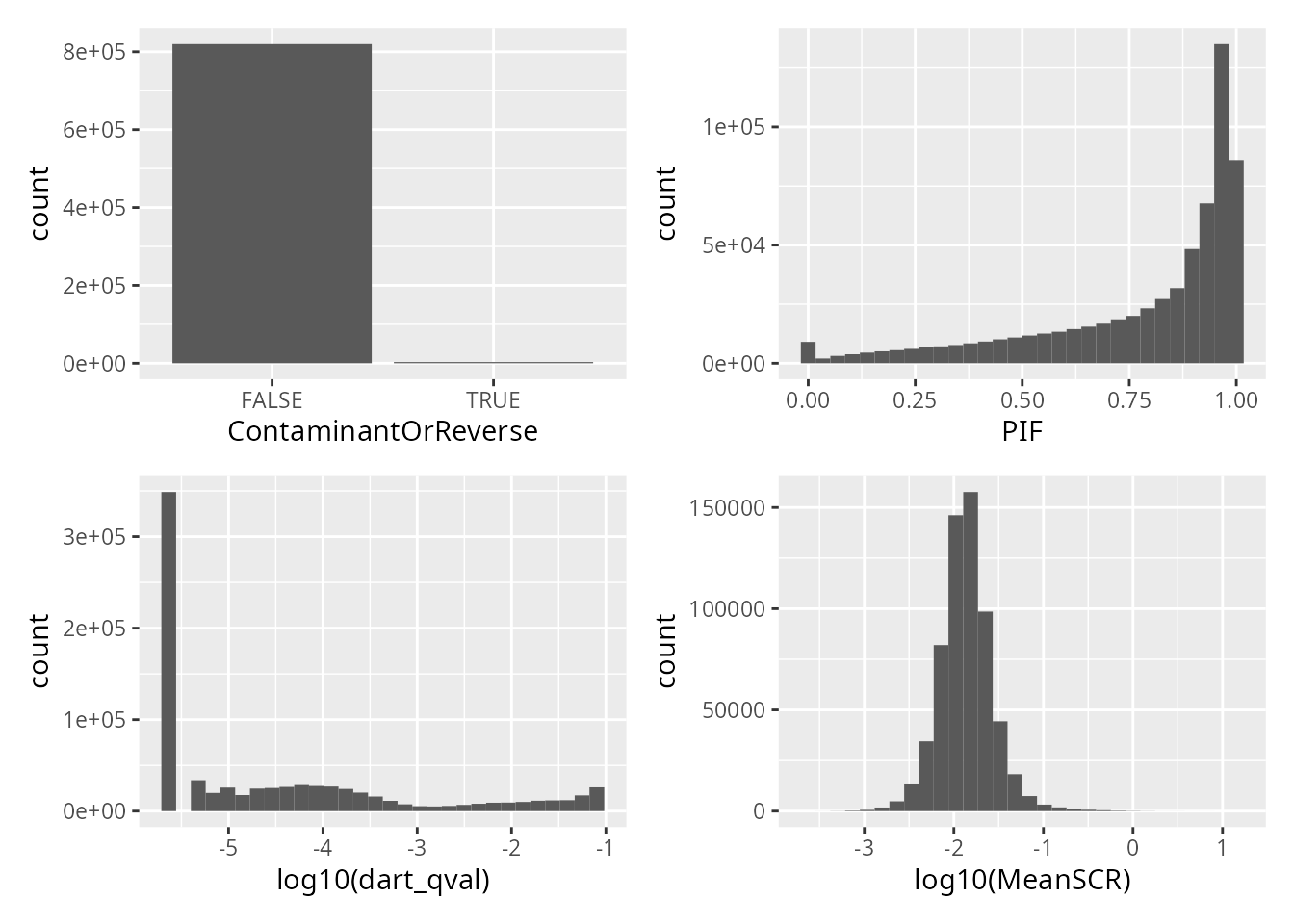

We filter and keep the features that pass the quality control criteria.

leduc <- filterFeatures(
    leduc, ~ Reverse != "+" &
        Potential.contaminant != "+" &
        !grepl("REV|CON", Leading.razor.protein) &
        !is.na(PIF) & PIF > 0.6 &
        dart_qval < 0.01 &
        !is.na(MeanSCR) & MeanSCR < 0.05
)
## 'Reverse' found in 134 out of 134 assay(s)
## 'Potential.contaminant' found in 134 out of 134 assay(s)
## 'Leading.razor.protein' found in 134 out of 134 assay(s)
## 'PIF' found in 134 out of 134 assay(s)
## 'dart_qval' found in 134 out of 134 assay(s)
## 'MeanSCR' found in 134 out of 134 assay(s)

Sample quality control

Similarly to the features, we also remove low-quality cells. The quality control criteria are:

We remove samples with low number of detected peptides. The criterion is computed as follows:

leduc <- countUniqueFeatures(
    leduc, i = names(leduc), groupBy = "Sequence",
    colDataName = "NumberPeptides"
)

We remove samples with low median intensity. The metric (note we will later use it for normalization) is computed as follows:

MedianIntensity <- lapply(experiments(leduc), function(x) {
    out <- colMedians(log(assay(x)), na.rm = TRUE)
    names(out) <- colnames(x)
    out
})
names(MedianIntensity) <- NULL
MedianIntensity <- unlist(MedianIntensity)
colData(leduc)[names(MedianIntensity), "MedianIntensity"] <- MedianIntensity

We remove the samples that have a high median coefficients of variation (CV). The CV is computed within each sample, by grouping the peptides that belong to the same protein or protein group. This is computed as follows:

leduc <- medianCVperCell(
    leduc, i = names(leduc), groupBy = "Leading.razor.protein.symbol",
    nobs = 3, na.rm = TRUE, colDataName = "MedianCV", norm = "SCoPE2"
)
## Warning in medianCVperCell(leduc, i = names(leduc), groupBy = "Leading.razor.protein.symbol", : The median CV could not be computed for one or more samples. You may want to try a smaller value for 'nobs'.

We also remove the samples that are not single cells because we will no longer need them.

We plot the metrics used to perform sample quality control.

ggplot(data.frame(colData(leduc))) +
    aes(
        y = MedianIntensity,
        x = NumberPeptides,
        color = MedianCV,
        shape = SampleType
    ) +
    geom_point(size = 2) +
    scale_color_continuous(type = "viridis")
## Warning: Removed 2 rows containing missing values (`geom_point()`).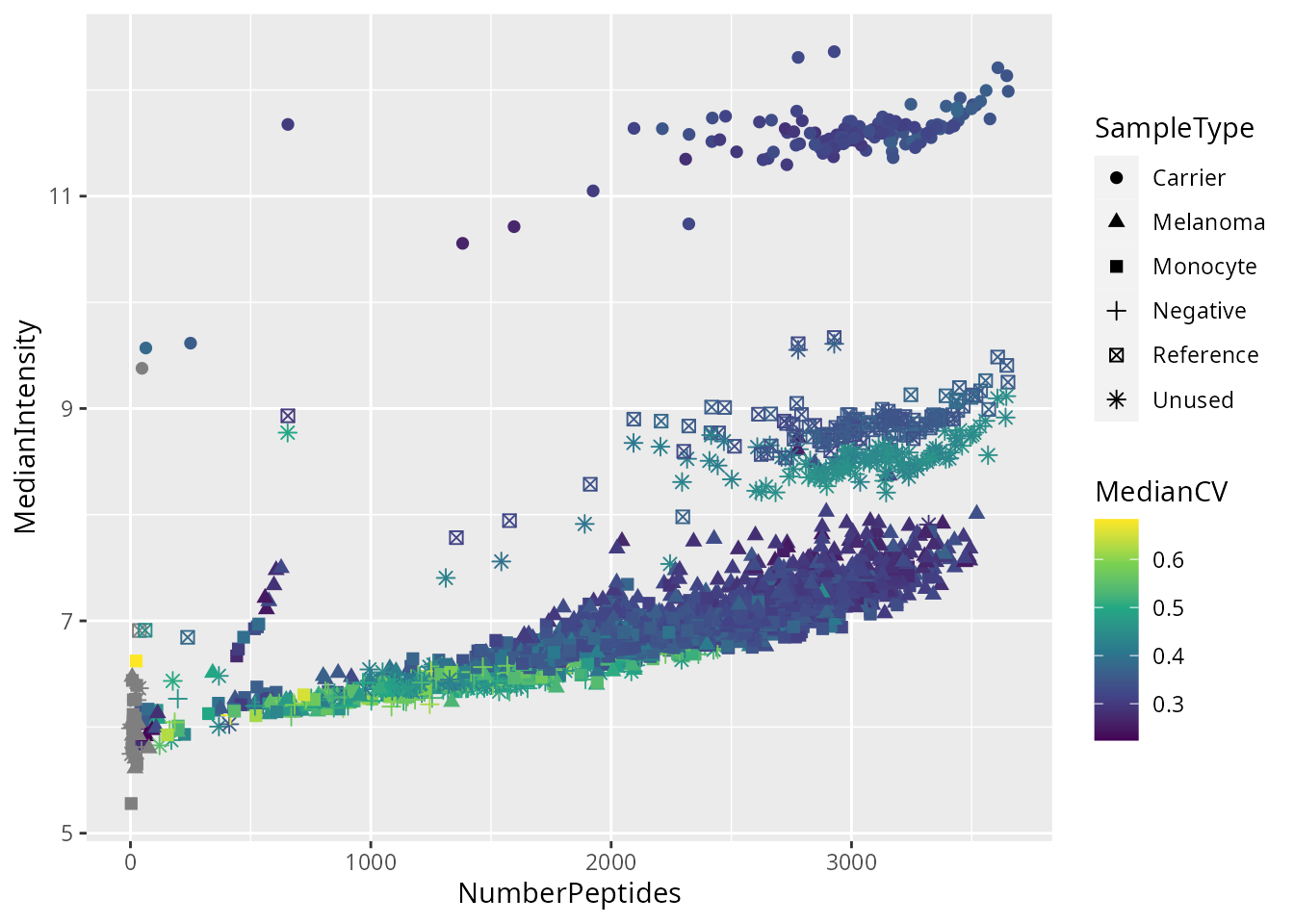

We apply the filter and keep only single cells that pass the quality control.

passQC <- !is.na(leduc$MedianCV) & leduc$MedianCV < 0.6 &
    leduc$MedianIntensity > 6 & leduc$MedianIntensity < 8 &
    leduc$NumberPeptides > 750 &
    grepl("Mono|Mel", leduc$SampleType)
leduc <- subsetByColData(leduc, passQC)

Peptide data assembly

For now each MS acquisition run is stored separately in an assay. We here combine these assays in one. The issue is that PSMs are specific to each run. We therefore aggregate the PSMs to peptides.

peptideAssays <- paste0("peptides_", names(leduc))
leduc <- aggregateFeatures(leduc,
                           i = names(leduc),
                           fcol = "Sequence",
                           name = peptideAssays,
                           fun = colMedians,
                           na.rm = TRUE)

Next to that, we must adapt the peptide to protein mapping. When joining all assay, we will only keep the feature annotations that have the common data. However, some peptide sequences map to one protein in one run and to another protein in another run. Hence, the protein name is not constant for all peptides and is removed during joining. It is important we keep the protein sequence in the rowData, in case we later want to aggregate, model or infer protein level quantification.

ppMap <- rbindRowData(leduc, i = grep("^pep", names(leduc))) %>%
    data.frame %>%
    group_by(Sequence) %>%
    ## The majority vote happens here
    mutate(Leading.razor.protein.symbol =
               names(sort(table(Leading.razor.protein.symbol),
                          decreasing = TRUE))[1],
           Leading.razor.protein.id =
               names(sort(table(Leading.razor.protein.id),
                          decreasing = TRUE))[1]) %>%
    dplyr::select(Sequence, Leading.razor.protein.symbol, Leading.razor.protein.id) %>%
    dplyr::filter(!duplicated(Sequence, Leading.razor.protein.symbol))
consensus <- lapply(peptideAssays, function(i) {
    ind <- match(rowData(leduc)[[i]]$Sequence, ppMap$Sequence)
    DataFrame(Leading.razor.protein.symbol =
                  ppMap$Leading.razor.protein.symbol[ind],
              Leading.razor.protein.id = 
                  ppMap$Leading.razor.protein.id[ind])
})
names(consensus) <- peptideAssays
rowData(leduc) <- consensus

The data can now be joined.

leduc <- joinAssays(leduc, i = peptideAssays, 
                    name = "peptides")

Finally, we also convert uniprot protein identifier to gene symbols.

proteinIds <- rowData(leduc)[["peptides"]]$Leading.razor.protein.id
proteinConversionDf <- transcripts(
    EnsDb.Hsapiens.v86, 
    columns = "gene_name",
    return.type = "data.frame",
    filter = UniprotFilter(proteinIds)
)
matchedIndex <- match(proteinIds, proteinConversionDf$uniprot_id)
geneName <- proteinConversionDf$gene_name[matchedIndex]
rowData(leduc)[["peptides"]]$gene <- geneName

Log-transformation

We log2-transform the quantification data.

leduc <- logTransform(leduc, i = "peptides", name = "peptides_log")

Here is an overview of the data processing:

plot(leduc)
## Warning in plot.QFeatures(leduc): The QFeatures object contains many assays.
## You may want to consider creating an interactive plot (set 'interactive =
## TRUE')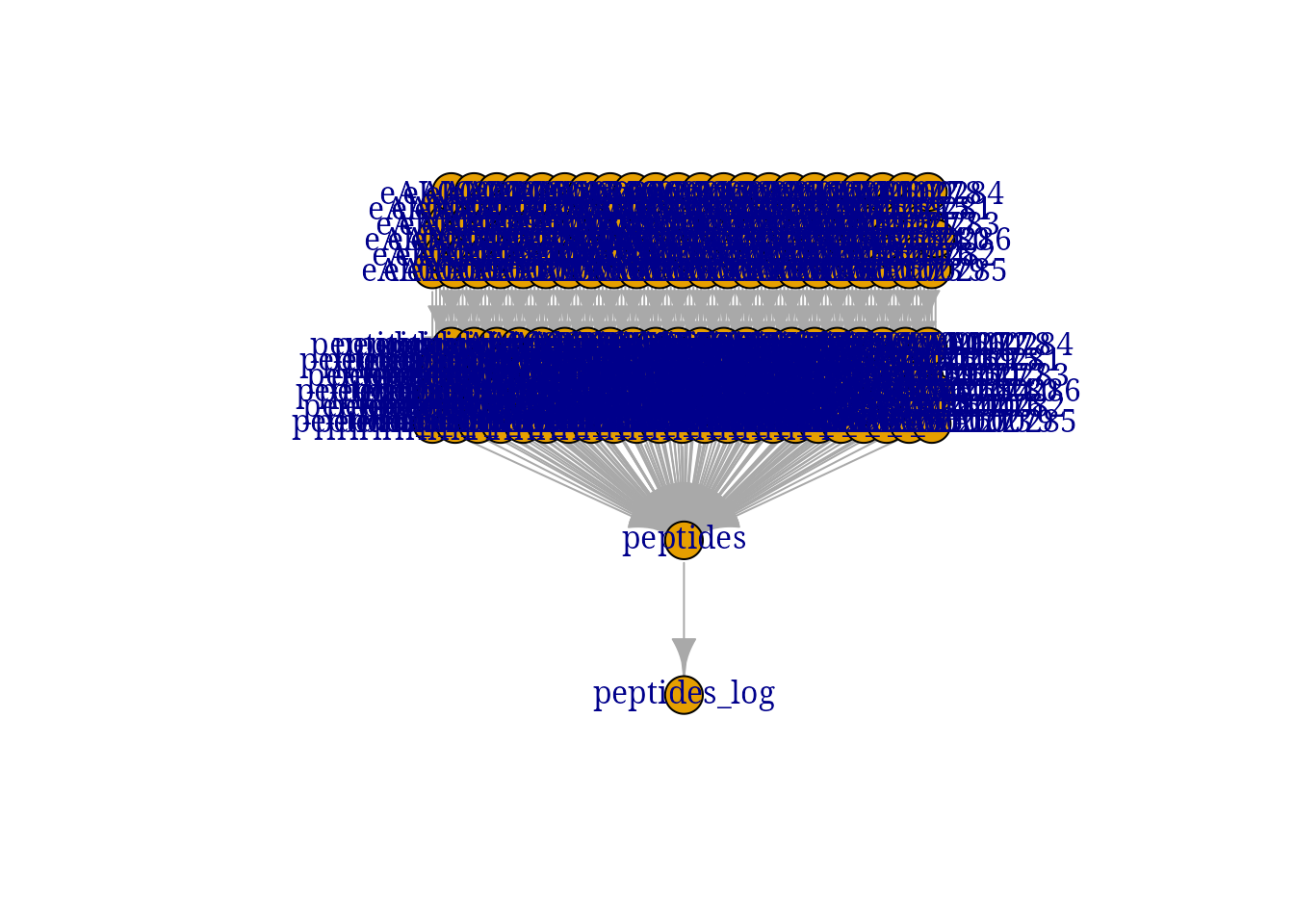

Data modelling

Model the data using the linear regression model implemented in scp. The model is applied on a SingleCellExperiment so we extract it from the processed data set along with the colData

sce <- getWithColData(leduc, "peptides_log")

First, we must specify which variables to include in the model. We here include 4 variables:

MedianIntensity: this is the normalization factor used to correct for cell-specific technical differences.
Channel: this is used to correct for TMT effects.
Set: this is used to perform batch correction. We consider each acquisition run to be a batch.
SampleType: this is the biological variable of interest. It capture the difference between macrophages and monocytes

scpModelWorkflow() fits linear regression models to the data, where the model is adapted for each peptide depending on its pattern of missing values.

sce <- scpModelWorkflow(
    sce,
    formula = ~ 1 + ## intercept
        ## normalization
        MedianIntensity +
        ## batch effects
        Channel + Set + 
        ## biological variability
        SampleType
)

Once the model is prepared, we can explore the distribution of the n/p ratios.

scpModelFilterThreshold(sce) <- 3
scpModelFilterPlot(sce)
## To change the threshold, use:
## scpModelFilterThreshold(object, name) <- threshold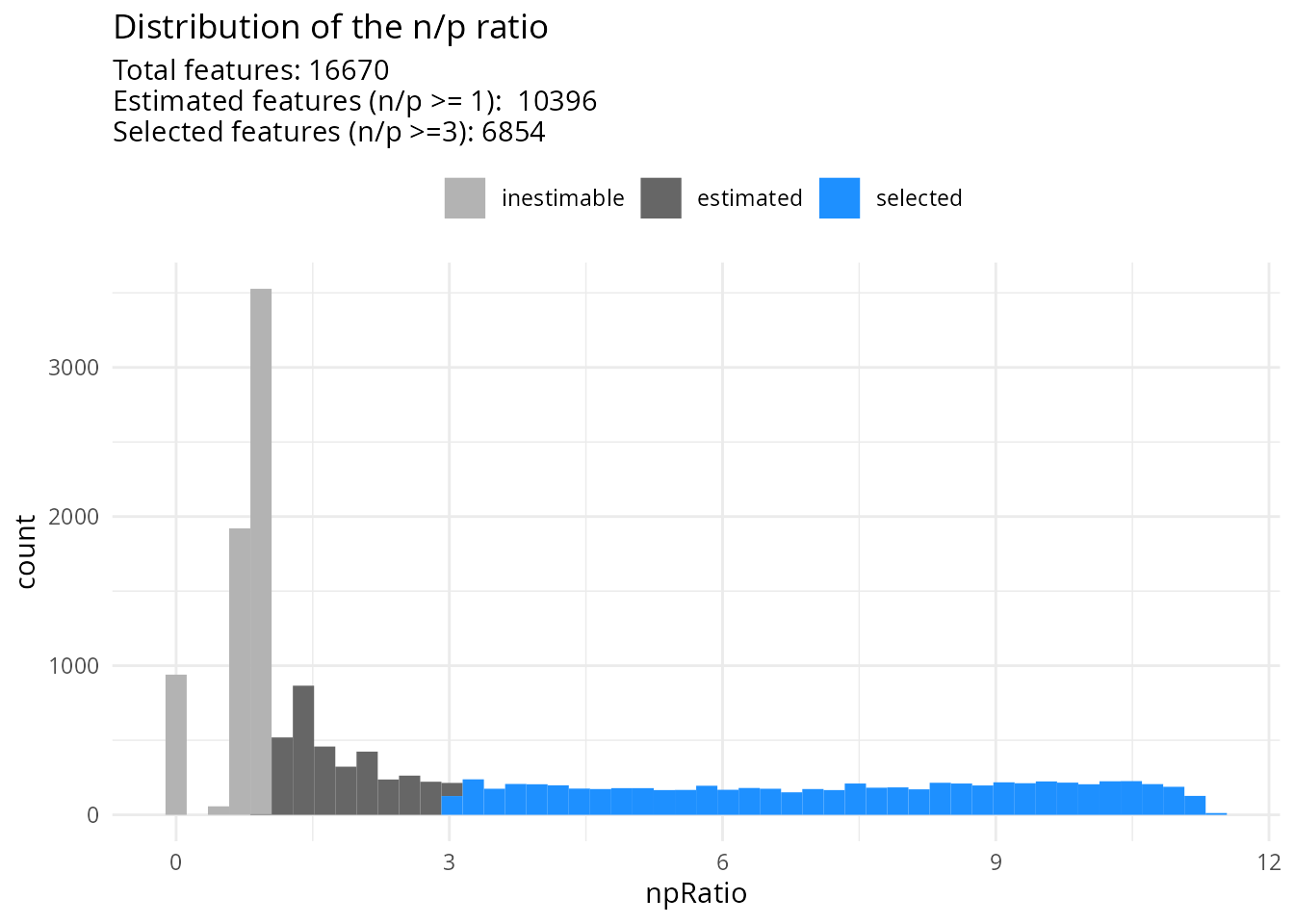

Many peptides do not have sufficient observations to estimate the model. We have chosen to continue the analysis with peptides that have \(n/p >= 3\). You could consider \(n/p\) a rough average of the number of replicates per parameter to fit (for categorical variables, the number of replicates per group). We recommend moving the threshold away from 1 to increase statistical power and remove noisy peptides. This comes of course at the cost of less peptides included in the analysis.

Model analysis

The model analysis consists of three steps:

Variance analysis
Differential abundance analysis
Component analysis

Variance analysis

The variance analysis explores the proportion of data captures by each variable in the model.

(vaRes <- scpVarianceAnalysis(sce))
## DataFrameList of length 5
## names(5): Residuals MedianIntensity Channel Set SampleType
vaRes[[1]]
## DataFrame with 6854 rows and 4 columns
##            feature        SS        df percentExplainedVar
##        <character> <numeric> <numeric>           <numeric>
## 1          GTLVQTK   428.956      1502            15.58356
## 2    NSNPALNDNL...   350.165      1357            25.62569
## 3    ITVTSEVPFS...   273.791      1365            22.35432
## 4    LVLVGDGGTG...   242.713      1471             9.67771
## 5          LVAQLYK   361.345      1175            36.60871
## ...            ...       ...       ...                 ...
## 6850 LIHPDEDISL...   75.4117       290             22.2277
## 6851 MQEHSDQVPV...  125.2367       494             45.1561
## 6852 HGAEVIDTPV...   38.6879       126             58.5003
## 6853 TETQEKNPLP...  404.3668       790             14.5120
## 6854 TLTTVQGIAD...   77.5062       253             66.6051

The results are a list of tables, one table for each variable. Each table reports for each peptide the variance captures (SS), the residual degrees of freedom for estimating the variance (df) and the percentage of total variance explained (percentExplainedVar). To better explore the results, we add the annotations available in the rowData.

vaRes <- scpAnnotateResults(
    vaRes, rowData(sce), by = "feature", by2 = "Sequence"
)

By default, we explore the variance for all peptides combined:

scpVariancePlot(vaRes)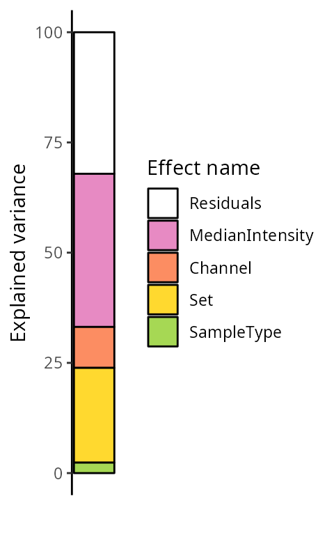

We explore the top 20 peptides that are have the highest percentage of variance explained by the biological variable (top) or by the batch variable (bottom).

scpVariancePlot(
    vaRes, top = 20, by = "percentExplainedVar", effect = "SampleType",
    decreasing = TRUE, combined = FALSE
) +
    scpVariancePlot(
    vaRes, top = 20, by = "percentExplainedVar", effect = "Set",
    decreasing = TRUE, combined = FALSE
) +
    plot_layout(ncol = 1, guides = "collect")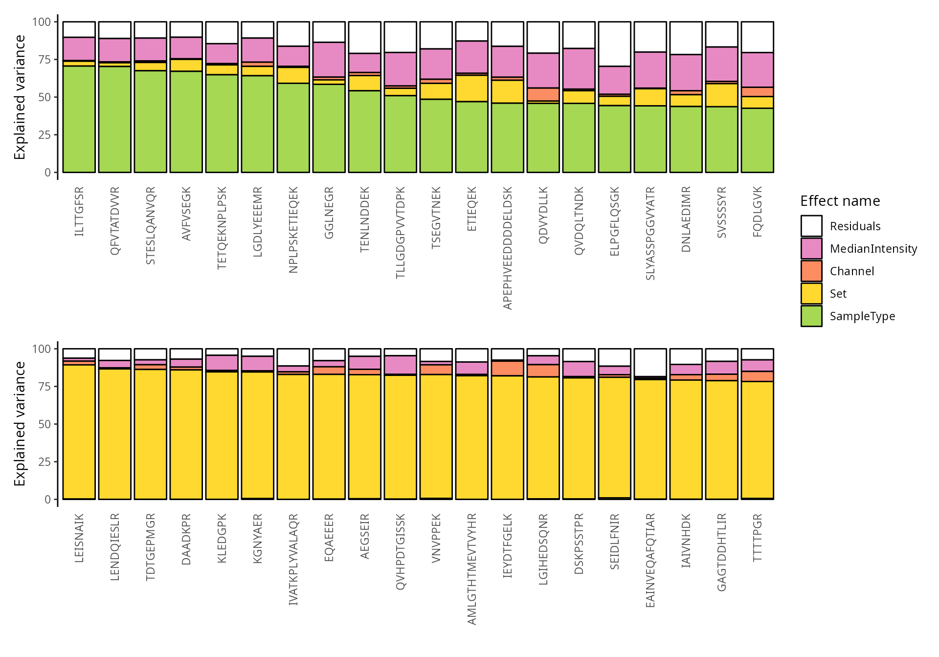

We can also group these peptide according to their protein. We simply need to provide the fcol argument.

scpVariancePlot(
    vaRes, top = 20, by = "percentExplainedVar", effect = "SampleType",
    decreasing = TRUE, combined = FALSE, fcol = "gene"
) +
    scpVariancePlot(
    vaRes, top = 20, by = "percentExplainedVar", effect = "Set",
    decreasing = TRUE, combined = FALSE, fcol = "gene"
) +
    plot_layout(ncol = 1, guides = "collect")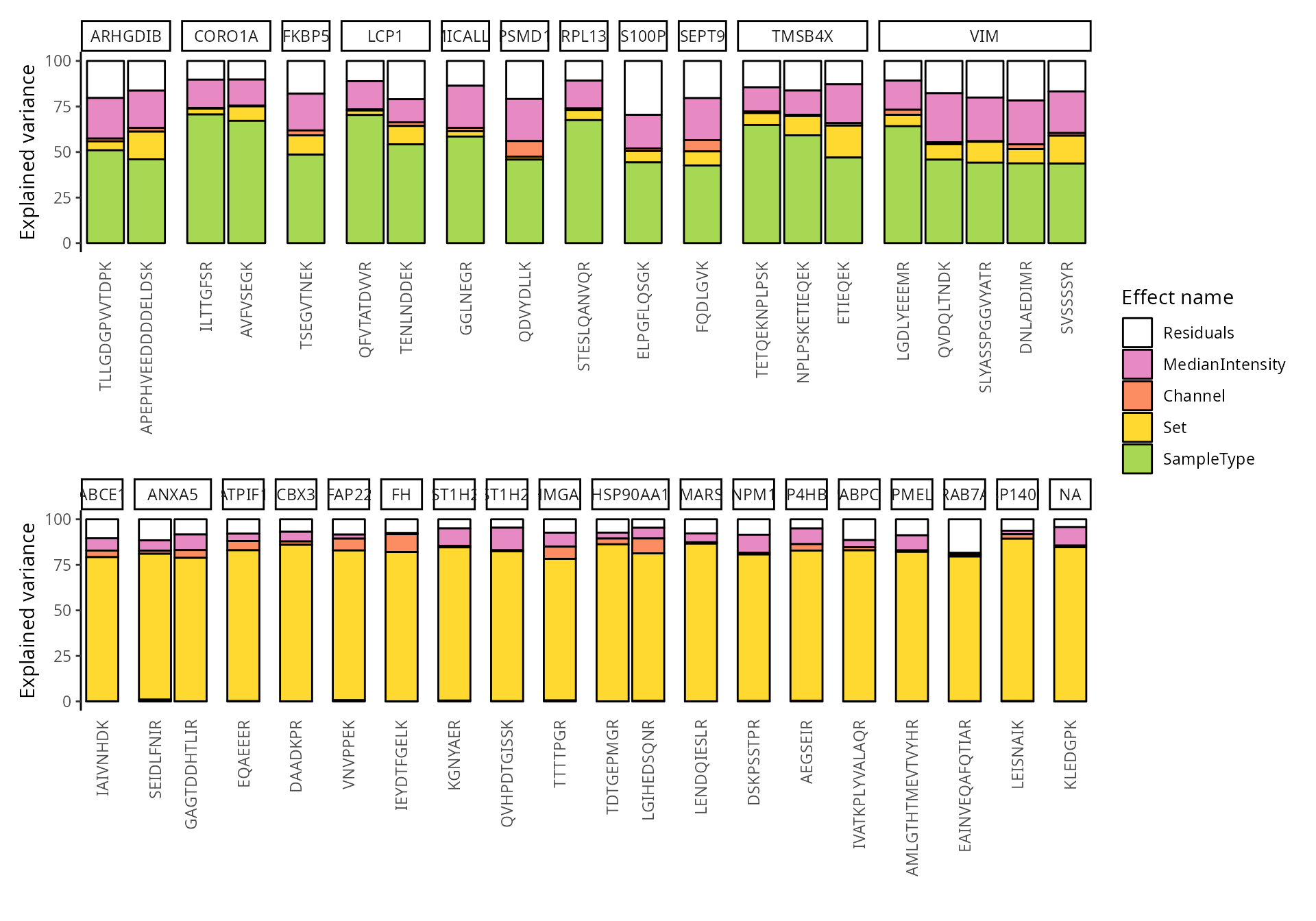

Differential abundance analysis

Next, we explore the model output to understand the differences between melanoma cells and monocytes. The difference of interest is specified using the contrast argument. The first element points to the variable to test and the two following element are the groups of interest to compare. You can provide multiple contrast in a list.

(daRes <- scpDifferentialAnalysis(
    sce, contrast = list(c("SampleType", "Melanoma", "Monocyte"))
))
## List of length 1
## names(1): SampleType_Melanoma_vs_Monocyte
daRes[[1]]
## DataFrame with 6854 rows and 7 columns
##            feature   Estimate        SE        Df tstatistic       pvalue
##        <character>  <numeric> <numeric> <numeric>  <numeric>    <numeric>
## 1          GTLVQTK -0.2348267 0.0461710      1502   -5.08602  4.11671e-07
## 2    NSNPALNDNL... -0.2964675 0.0476322      1357   -6.22410  6.44196e-10
## 3    ITVTSEVPFS...  0.1699631 0.0422754      1365    4.02038  6.12828e-05
## 4    LVLVGDGGTG... -0.0575517 0.0359411      1471   -1.60128  1.09529e-01
## 5          LVAQLYK  0.2392563 0.0586715      1175    4.07790  4.85057e-05
## ...            ...        ...       ...       ...        ...          ...
## 6850 LIHPDEDISL...  0.1568293 0.1001117       290   1.566543  1.18312e-01
## 6851 MQEHSDQVPV... -0.0352213 0.0803697       494  -0.438241  6.61403e-01
## 6852 HGAEVIDTPV...  0.0925308 0.1753991       126   0.527545  5.98743e-01
## 6853 TETQEKNPLP... -2.8525348 0.1002023       790 -28.467765 3.09874e-123
## 6854 TLTTVQGIAD...  0.1569952 0.1299189       253   1.208409  2.28018e-01
##              padj
##         <numeric>
## 1     3.30397e-06
## 2     6.93142e-09
## 3     3.63979e-04
## 4     2.69653e-01
## 5     2.91886e-04
## ...           ...
## 6850  2.84930e-01
## 6851  8.40398e-01
## 6852  8.01521e-01
## 6853 2.35986e-120
## 6854  4.57104e-01

Similarly to variance analysis, the results are a list of tables, one table for each contrast. Each table reports for each peptide the estimated difference between the two groups, the standard error associated to the estimation, the degrees of freedom, the t-statistics, the associated p-value and the p-value FDR-adjusted for multiple testing across all peptides. Again, to better explore the results, we add the annotations available in the rowData.

daRes <- scpAnnotateResults(
    daRes, rowData(sce), 
    by = "feature", by2 = "Sequence"
)

We then visualize the results using a volcano plot. The function below return a volcano plot for each contrast.

scpVolcanoPlot(daRes)
## $SampleType_Melanoma_vs_Monocyte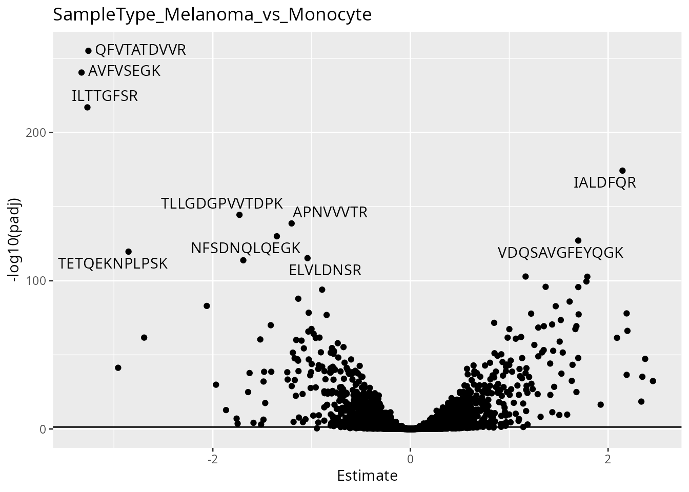

To help interpretation of the results, we will label the peptides with their protein name. Also we increase the number of labels shown on the plot. Finally, we can add colors to the plot. For instance, let’s explore the impact of the number of observations using the \(n/p\) ratio. We create a new annotation table, add it to the results and redraw the plot. The \(n/p\) ratio is retrieved using scpModelFilterNPRatio

np <- scpModelFilterNPRatio(sce)
daRes <- scpAnnotateResults(
    daRes, data.frame(feature = names(np), npRatio = np), 
    by = "feature"
)
scpVolcanoPlot(
    daRes, top = 30, textBy = "gene", 
    pointParams = list(aes(colour = npRatio))
)
## $SampleType_Melanoma_vs_Monocyte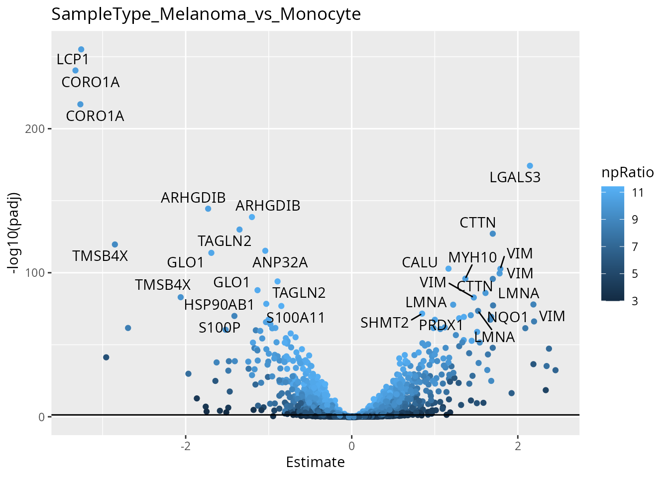

As expected, higher number of observations (higher \(n/p\)) lead to increased statistical power and hence to more significant results.

Proteins such as VIM, LGALS3, CALU, LMNA, CTTN, are more abundant in melanoma cells compared to monocytes. On the other hand, proteins such as LCP1, CORO1A, ARHGDIB, TMSB4X are more abundant in monocytes compared to melanoma cells.

Finally, we offer functionality to report results at the protein level.

scpDifferentialAggregate(daRes, fcol = "gene") |> 
    scpVolcanoPlot(top = 30, textBy = "gene")
## $SampleType_Melanoma_vs_Monocyte
## Warning: ggrepel: 3 unlabeled data points (too many overlaps). Consider
## increasing max.overlaps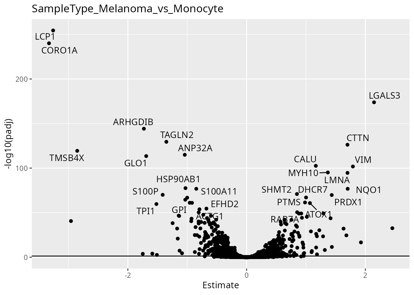

Component analysis

Finally, we perform component analysis to link the modelled effects to the cellular heterogeneity. We here run an APCA+ (extended ANOVA-simultaneous principal component analysis) for the sample type effect. In other words, we perform a PCA on the data that is capture by the sample type variable along with the residuals (unmodelled data).

(caRes <- scpComponentAnalysis(
    sce, ncomp = 2, method = "APCA", effect = "SampleType"
))
## [1] "APCA"
## [1] "SampleType"
## List of length 2
## names(2): bySample byFeature

The results are contained in a list with 2 elements. bySample contains the PC scores, that is the component results in sample space. byFeature contains the eigenvectors, that is the component results in feature space.

caRes$bySample
## List of length 3
## names(3): unmodelled residuals APCA_SampleType

Each of the two elements contains components results for the data before modelling (unmodelled), for the residuals or for the APCA on the sample type variable (APCA_SampleType).

caRes$bySample[[1]]
## DataFrame with 1656 rows and 3 columns
##                    PC1        PC2          cell
##              <numeric>  <numeric>   <character>
## eAL00219RI5   34.82634    25.4084 eAL00219RI...
## eAL00219RI6   27.30071    28.3922 eAL00219RI...
## eAL00219RI7   10.85533    29.7354 eAL00219RI...
## eAL00219RI8    2.81552    28.9838 eAL00219RI...
## eAL00219RI9   47.84411    29.4004 eAL00219RI...
## ...                ...        ...           ...
## wAL00286RI12 -32.95100  -3.641834 wAL00286RI...
## wAL00286RI14 -36.19707  -0.283055 wAL00286RI...
## wAL00286RI16   9.79076 -13.134253 wAL00286RI...
## wAL00286RI17   2.63224 -16.199820 wAL00286RI...
## wAL00286RI18  -1.84038 -18.643383 wAL00286RI...

Each elements is a table with the computed componoents. Let’s explore the component analysis results in cell space. Similarly to the previous explorations, we annotate the results.

caResCells <- caRes$bySample
sce$cell <- colnames(sce)
caResCells <- scpAnnotateResults(caResCells, colData(sce), by = "cell")

We then generate the component plot, colouring by SampleType. To assess the impact of batch effects, we shape the points according to the plate batch (cf intro) as well.

scpComponentPlot(
    caResCells,
    pointParams = list(aes(colour = SampleType, shape = lcbatch))
) |>
    wrap_plots() +
    plot_layout(guides = "collect")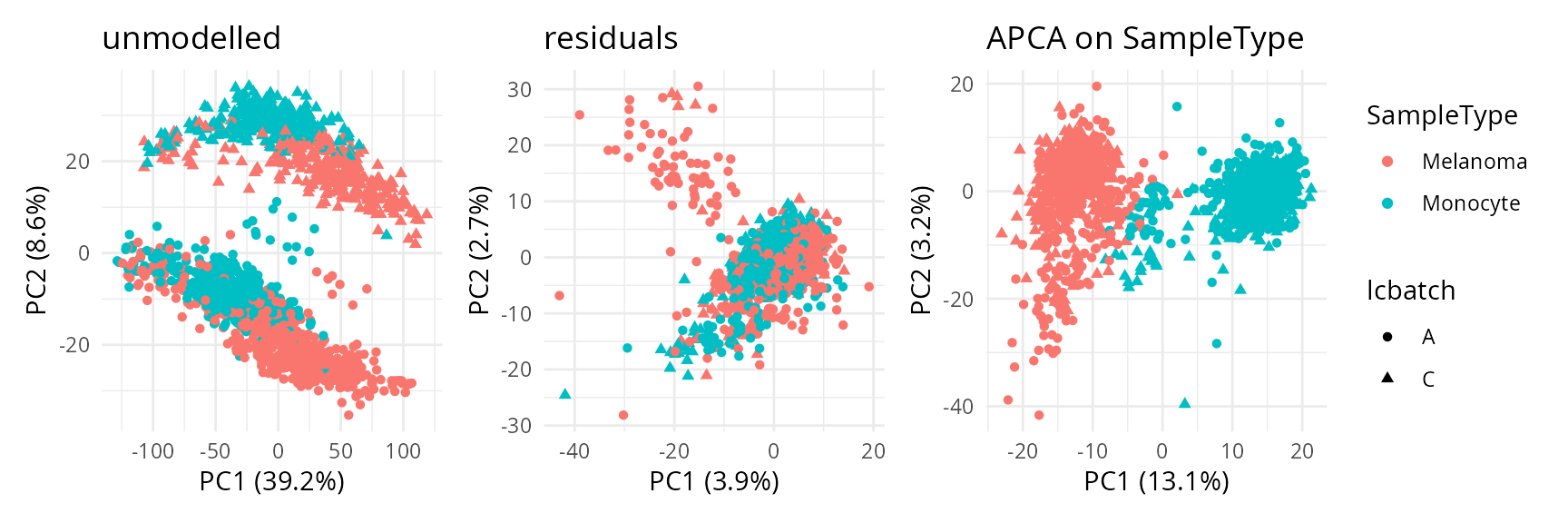

While the data before modelling is mainly driven by batch effects, the APCA clearly separates the two cell populations. Interestingly, the PCA on the residuals suggests that there is a small subpopulation that we did not model. We will explore this later during downstream analysis.

We use the same approach to explore the component results in feature space.

caResPeps <- caRes$byFeature
caResPeps <- scpAnnotateResults(
    caResPeps, rowData(sce), by = "feature", by2 = "Sequence"
)

We plot the compenents in peptide-space.

plCApeps <- scpComponentPlot(
    caResPeps, pointParams = list(size = 0.8, alpha = 0.4)
)
wrap_plots(plCApeps)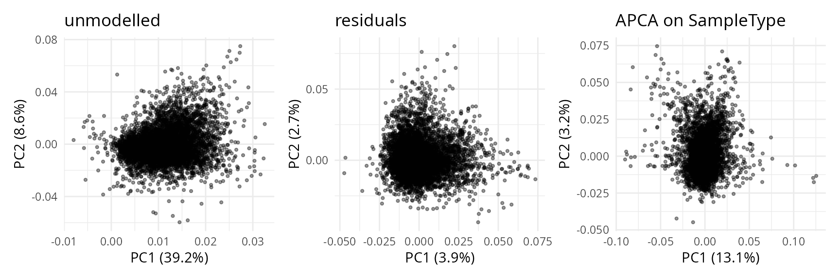

We can also combine the exploration of the components in cell and peptide space. This is possible thanks to biplots.

biplots <- scpComponentBiplot(
    caResCells, caResPeps, 
    pointParams = list(aes(colour = SampleType, shape = lcbatch)),
    labelParams = list(size = 1.5, max.overlaps = 20),
    textBy = "gene", top = 20
)
wrap_plots(biplots, guides = "collect")
## Warning: Removed 4 rows containing missing values
## (`geom_label_repel()`).
## Warning: ggrepel: 16 unlabeled data points (too many overlaps). Consider
## increasing max.overlaps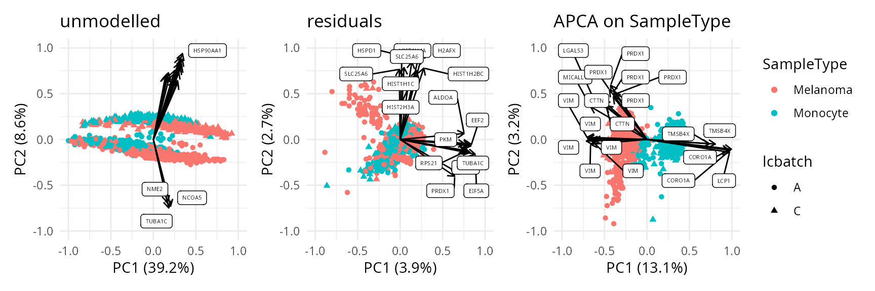

Finally, we offer functionality to aggregate the results at the protein level instead of the peptide level.

caResProts <- scpComponentAggregate(caResPeps, fcol = "gene")
## Components may no longer be orthogonal after aggregation.
biplots <- scpComponentBiplot(
    caResCells, caResProts, 
    pointParams = list(aes(colour = SampleType, shape = lcbatch)),
    labelParams = list(size = 1.5, max.overlaps = 20),
    textBy = "gene", top = 20
)
wrap_plots(biplots, guides = "collect")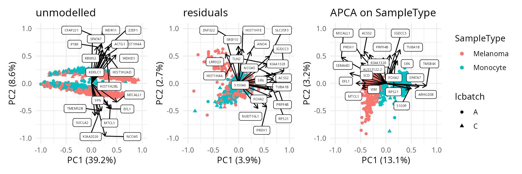

Interactive visualisation with iSEE

You can manually explore the data through an interactive interface thanks to using the iSEE:

library("iSEE")
iSEE(sce)

Downstream analysis

The final step in this analyses in the identification of the small melanoma subpopulation. To achieve this, we perform an APCA+ with more components to capture most of the variability. Then, we cluster the cells to highlight the subpopulations. We then retrieve the batch corrected data. Finally, we run a new model on the melanoma data to find marker proteins that are strongly differentially abundant between the two cell subpopulations.

Clustering

Before applying the cluster algorithm, we compute the 20 first APCA+ components on the sample type. We limit the PCA algorithm to 50 iterations to avoid an overly long run and will not compute the PCA for the unmodelled data and the residuals because we won’t use it during the downstream analysis.

apcaSampleType <- scpComponentAnalysis(
    sce, ncomp = 20, method = "APCA", effect = "SampleType", 
    residuals = FALSE, unmodelled = FALSE, maxiter = 50
)$bySample$APCA_SampleType
## [1] "APCA"
## [1] "SampleType"

The resulting components are stored in the SingleCellExperiment object.

pcCols <- grep("^PC", colnames(apcaSampleType))
reducedDim(sce, "APCA") <- apcaSampleType[, pcCols]

Next, we visualize these 20 components by further decreasing the dimensions using t-SNE.

set.seed(1234)
sce <- runTSNE(sce, dimred = "APCA")
plotTSNE(sce)

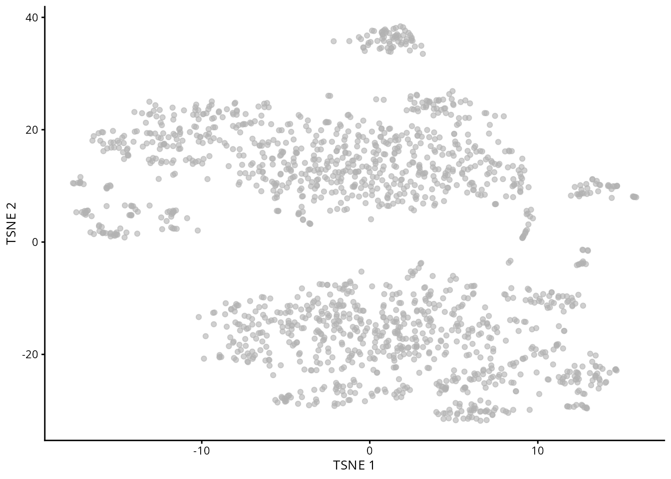
Finally, we cluster cells based on a shared nearest neighbour embedding followed by community detection using the Louvain algorithm.

algo <- SNNGraphParam(k = 30, type = "rank", cluster.fun = "louvain")
sce$Cluster <- clusterRows(
    reducedDim(sce, "APCA"), BLUSPARAM = algo
)
plotTSNE(sce, colour_by = "Cluster")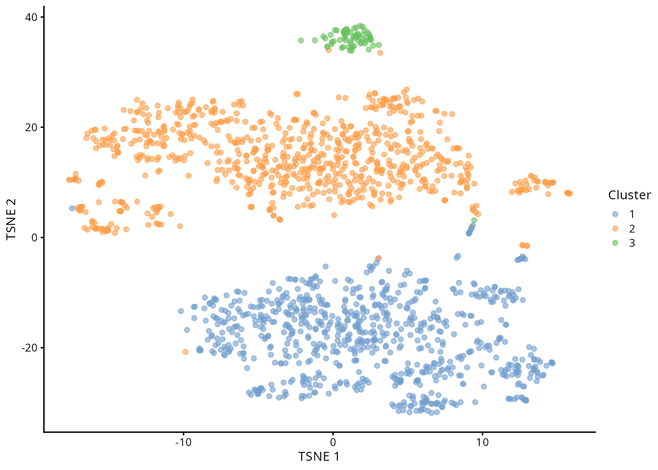

The clustering retrieved 3 cell population, more or less splitting the melanoma cells in 2 subpopulation. Note that \(k\) was arbitrarily set to 30. A thorough analysis would optimize K based on an objective criterion, such as maximizing the average silhouette width.

Below is an overview of the unsupervised clusters against the known annotations provided by the authors after thorough investigation.

table(
    Cluster = sce$Cluster, 
    Population = paste(sce$SampleType, sce$MelanomaSubCluster)
)
##        Population
## Cluster Melanoma A Melanoma B Melanoma NA Monocyte NA
##       1          2          0           0         769
##       2        691          4          70          55
##       3          1         53          11           0

We annotate the the unsupervised clusters using the available annotations.

sce$Cluster <- recode(sce$Cluster, "1" = "Monocyte", "2" = "Melanoma A", "3" = "Melanoma B")

Batch correction

Based on the model fitted in the previous section, we generate batch-corrected data, that is data with only the effect of cell type and the residual data. We also remove the intercept.

(scebr <- scpRemoveBatchEffect(
    sce, effects = c("Set", "Channel", "MedianIntensity"),
    intercept = TRUE
))
## class: SingleCellExperiment 
## dim: 6854 1656 
## metadata(0):
## assays(1): ''
## rownames(6854): GTLVQTK NSNPALNDNLEK ... TETQEKNPLPSK TLTTVQGIADDYDK
## rowData names(6): Sequence Reverse ... Leading.razor.protein.symbol
##   gene
## colnames(1656): eAL00219RI5 eAL00219RI6 ... wAL00286RI17 wAL00286RI18
## colData names(13): Set Channel ... cell Cluster
## reducedDimNames(0):
## mainExpName: NULL
## altExpNames(0):

Note that the batch-corrected data still contain missing values.

Marker proteins

To identify markers proteins, we run a differential abundance analysis as presented in the previous section. We create a new model, focusing only on melanoma data as we don’t want to compare subpopulations with monocytes.

sceMel <- scebr[, scebr$SampleType == "Melanoma"]
sceMel <- scpModelWorkflow(sceMel, formula = ~ 1 + Cluster)

We then apply the same procedure as described above.

daRes <- scpDifferentialAnalysis(sceMel, contrasts = list(c(
    "Cluster", "Melanoma A", "Melanoma B"
)))
daRes <- scpAnnotateResults(
    daRes, rowData(sceMel), 
    by = "feature", by2 = "Sequence"
)
scpVolcanoPlot(daRes, top = 100, textBy = "gene")
## $Cluster_Melanoma.A_vs_Melanoma.B
## Warning: Removed 234 rows containing missing values (`geom_point()`).
## Warning: Removed 2 rows containing missing values (`geom_text_repel()`).
## Warning: ggrepel: 56 unlabeled data points (too many overlaps). Consider
## increasing max.overlaps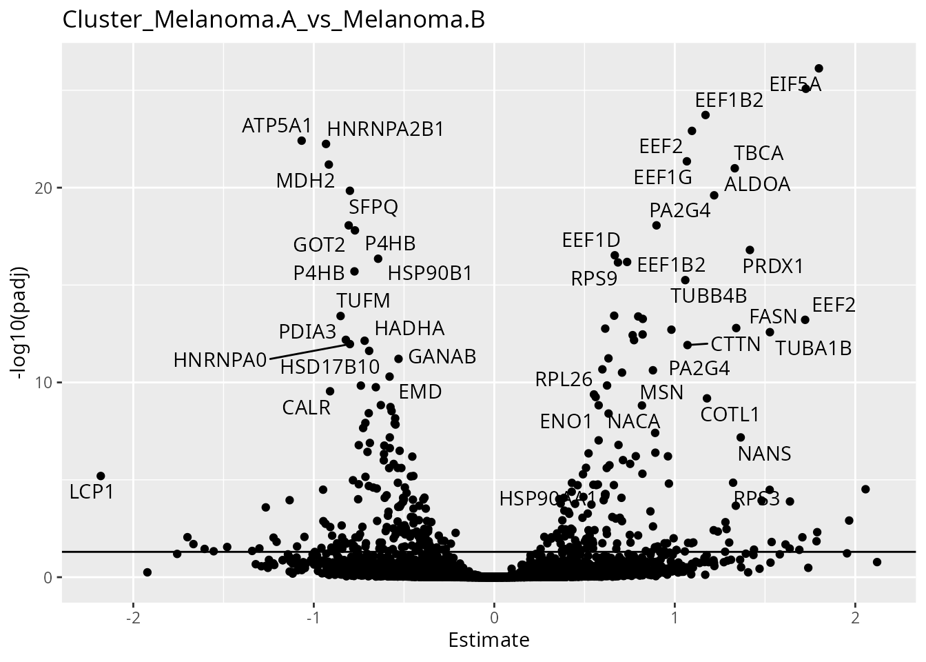

Interestingly, subpopulation be is characterized by higher abundances of MATR3 and SFPQ (involved in response to DNA double-strand break), P4HB and PDIA3 (involved in disulfide bond rearrangement). On the other hand, melanoma subpopulation A shows more elongation factors (EEF1B3, EEF2, ), proteins associated with tubulin (TBCA, TUBB4B, TUBA1C, …) or proliferation control proteins (PA2G4, ENO1). This is in line with previous findings from the authors.

Session information

R Under development (unstable) (2023-07-27 r84768)
Platform: x86_64-pc-linux-gnu
Running under: Ubuntu 23.04

Matrix products: default
BLAS:   /usr/lib/x86_64-linux-gnu/blas/libblas.so.3.11.0 
LAPACK: /usr/lib/x86_64-linux-gnu/lapack/liblapack.so.3.11.0

locale:
 [1] LC_CTYPE=en_US.UTF-8       LC_NUMERIC=C              
 [3] LC_TIME=en_US.UTF-8        LC_COLLATE=en_US.UTF-8    
 [5] LC_MONETARY=en_US.UTF-8    LC_MESSAGES=en_US.UTF-8   
 [7] LC_PAPER=en_US.UTF-8       LC_NAME=C                 
 [9] LC_ADDRESS=C               LC_TELEPHONE=C            
[11] LC_MEASUREMENT=en_US.UTF-8 LC_IDENTIFICATION=C       

time zone: Europe/Prague
tzcode source: system (glibc)

attached base packages:
[1] stats4    stats     graphics  grDevices utils     datasets  methods  
[8] base     

other attached packages:
 [1] scater_1.31.0               scuttle_1.13.0             
 [3] SingleCellExperiment_1.25.0 bluster_1.13.0             
 [5] dplyr_1.1.3                 EnsDb.Hsapiens.v86_2.99.0  
 [7] ensembldb_2.27.0            AnnotationFilter_1.27.0    
 [9] GenomicFeatures_1.55.1      AnnotationDbi_1.65.2       
[11] patchwork_1.1.3             ggplot2_3.4.4              
[13] scpdata_1.9.2               ExperimentHub_2.11.0       
[15] AnnotationHub_3.11.0        BiocFileCache_2.11.1       
[17] dbplyr_2.4.0                scp_1.11.3                 
[19] QFeatures_1.13.0            MultiAssayExperiment_1.29.0
[21] SummarizedExperiment_1.33.0 Biobase_2.63.0             
[23] GenomicRanges_1.55.1        GenomeInfoDb_1.39.0        
[25] IRanges_2.37.0              S4Vectors_0.41.1           
[27] BiocGenerics_0.49.1         MatrixGenerics_1.15.0      
[29] matrixStats_1.1.0           BiocStyle_2.31.0           

loaded via a namespace (and not attached):
  [1] later_1.3.1                   BiocIO_1.13.0                
  [3] bitops_1.0-7                  filelock_1.0.2               
  [5] tibble_3.2.1                  lpsymphony_1.31.0            
  [7] XML_3.99-0.15                 lifecycle_1.0.4              
  [9] rprojroot_2.0.4               lattice_0.22-5               
 [11] MASS_7.3-60.1                 magrittr_2.0.3               
 [13] sass_0.4.7                    rmarkdown_2.25               
 [15] jquerylib_0.1.4               yaml_2.3.7                   
 [17] metapod_1.11.0                httpuv_1.6.12                
 [19] cowplot_1.1.1                 MsCoreUtils_1.15.1           
 [21] DBI_1.1.3                     RColorBrewer_1.1-3           
 [23] abind_1.4-5                   zlibbioc_1.49.0              
 [25] Rtsne_0.16                    purrr_1.0.2                  
 [27] RCurl_1.98-1.13               rappdirs_0.3.3               
 [29] GenomeInfoDbData_1.2.11       ggrepel_0.9.4                
 [31] irlba_2.3.5.1                 pkgdown_2.0.7                
 [33] DelayedMatrixStats_1.25.0     codetools_0.2-19             
 [35] DelayedArray_0.29.0           xml2_1.3.5                   
 [37] tidyselect_1.2.0              farver_2.1.1                 
 [39] ScaledMatrix_1.11.0           viridis_0.6.4                
 [41] nipals_0.8                    GenomicAlignments_1.39.0     
 [43] jsonlite_1.8.7                BiocNeighbors_1.21.0         
 [45] ellipsis_0.3.2                systemfonts_1.0.5            
 [47] tools_4.4.0                   progress_1.2.2               
 [49] ragg_1.2.6                    Rcpp_1.0.11                  
 [51] glue_1.6.2                    BiocBaseUtils_1.5.0          
 [53] gridExtra_2.3                 SparseArray_1.3.0            
 [55] xfun_0.41                     withr_2.5.2                  
 [57] BiocManager_1.30.22           fastmap_1.1.1                
 [59] fansi_1.0.5                   digest_0.6.33                
 [61] rsvd_1.0.5                    R6_2.5.1                     
 [63] mime_0.12                     textshaping_0.3.7            
 [65] colorspace_2.1-0              biomaRt_2.59.0               
 [67] RSQLite_2.3.3                 utf8_1.2.4                   
 [69] tidyr_1.3.0                   generics_0.1.3               
 [71] rtracklayer_1.63.0            prettyunits_1.2.0            
 [73] httr_1.4.7                    S4Arrays_1.3.0               
 [75] pkgconfig_2.0.3               gtable_0.3.4                 
 [77] blob_1.2.4                    XVector_0.43.0               
 [79] htmltools_0.5.7               bookdown_0.36                
 [81] ProtGenerics_1.35.0           clue_0.3-65                  
 [83] scales_1.2.1                  png_0.1-8                    
 [85] knitr_1.45                    rjson_0.2.21                 
 [87] curl_5.1.0                    cachem_1.0.8                 
 [89] stringr_1.5.0                 BiocVersion_3.19.1           
 [91] parallel_4.4.0                vipor_0.4.5                  
 [93] restfulr_0.0.15               desc_1.4.2                   
 [95] pillar_1.9.0                  grid_4.4.0                   
 [97] vctrs_0.6.4                   slam_0.1-50                  
 [99] promises_1.2.1                BiocSingular_1.19.0          
[101] IHW_1.31.0                    beachmat_2.19.0              
[103] xtable_1.8-4                  cluster_2.1.4                
[105] beeswarm_0.4.0                evaluate_0.23                
[107] cli_3.6.1                     compiler_4.4.0               
[109] Rsamtools_2.19.2              rlang_1.1.2                  
[111] crayon_1.5.2                  labeling_0.4.3               
[113] fdrtool_1.2.17                fs_1.6.3                     
[115] ggbeeswarm_0.7.2              stringi_1.7.12               
[117] viridisLite_0.4.2             BiocParallel_1.37.0          
[119] munsell_0.5.0                 Biostrings_2.71.1            
[121] lazyeval_0.2.2                Matrix_1.6-1.1               
[123] hms_1.1.3                     sparseMatrixStats_1.15.0     
[125] bit64_4.0.5                   KEGGREST_1.43.0              
[127] shiny_1.7.5.1                 highr_0.10                   
[129] interactiveDisplayBase_1.41.0 igraph_1.5.1                 
[131] memoise_2.0.1                 bslib_0.5.1                  
[133] bit_4.0.5

Citation

citation("scp")
To cite the scp package in publications use:

  Vanderaa, Christophe, and Laurent Gatto. 2023.  Revisiting the Thorny
  Issue of Missing Values in Single-Cell Proteomics. Journal of
  Proteome Research 22 (9): 2775–84.

  Vanderaa Christophe and Laurent Gatto. The current state of
  single-cell proteomics data analysis. Current Protocols 3 (1): e658.;
  doi: https://doi.org/10.1002/cpz1.658 (2023).

  Vanderaa Christophe and Laurent Gatto. Replication of Single-Cell
  Proteomics Data Reveals Important Computational Challenges. Expert
  Review of Proteomics, 1–9 (2021).

To see these entries in BibTeX format, use 'print(<citation>,
bibtex=TRUE)', 'toBibtex(.)', or set
'options(citation.bibtex.max=999)'.

License

This vignette is distributed under a CC BY-SA license license.

christophe.vanderaa@uclouvain.be ↩︎

Christophe Vanderaa¹, Computational Biology, UCLouvain

Laurent Gatto, Computational Biology, UCLouvain

10 November 2023

Introduction

Packages and data

Minimal data processing

Cleaning data

Feature quality control

Sample quality control

Peptide data assembly

Log-transformation

Data modelling

Model analysis

Variance analysis

Differential abundance analysis

Component analysis

Interactive visualisation with iSEE

Downstream analysis

Clustering

Batch correction

Marker proteins

Session information

Citation

License

scplainer: reanalysis of the nPOP dataset (Leduc et al. 2022)

Christophe Vanderaa1, Computational Biology, UCLouvain

Laurent Gatto, Computational Biology, UCLouvain

10 November 2023

Introduction

Packages and data

Minimal data processing

Cleaning data

Feature quality control

Sample quality control

Peptide data assembly

Log-transformation

Data modelling

Model analysis

Variance analysis

Differential abundance analysis

Component analysis

Interactive visualisation with iSEE

Downstream analysis

Clustering

Batch correction

Marker proteins

Session information

Citation

License

Christophe Vanderaa¹, Computational Biology, UCLouvain