Automation and Visualization of Flow Cytometry Data Analysis Pipelines
Philippe Hauchamps
Laurent Gatto
Source:vignettes/CytoPipeline.Rmd
CytoPipeline.RmdAbstract
This vignette describes the functionality implemented in the
CytoPipeline package. CytoPipeline
provides support for automation and visualization of flow
cytometry data analysis pipelines. In the current state, the
package focuses on the pre-processing and quality control part.
This vignette is distributed under a CC BY-SA 4.0 license.
Installation
To install this package, start R and enter (uncommented):
# if (!require("BiocManager", quietly = TRUE))
#     install.packages("BiocManager")
#
# BiocManager::install("CytoPipeline")
Note that CytoPipeline imports ggplot2 (>= 3.4.1).
The version requirement is due to a bug in version 3.4.0., affecting
ggplot2::geom_hex().
Introduction
The CytoPipeline package provides infrastructure to
support the definition, run and standardized visualization of
pre-processing and quality control pipelines for flow cytometry data.
This infrastructure consists of two main S4 classes,
i.e. CytoPipeline and CytoProcessingStep, as
well as dedicated wrapper functions around selected third-party package
methods often used to implement these pre-processing steps.
In the following sections, we demonstrate how to create a
CytoPipeline object implementing a simple pre-processing
pipeline, how to run it and how to retrieve and visualize the results
after each step.
Example dataset
The example dataset that will be used throughout this vignette is derived from a reference public dataset accompanying the OMIP-021 (Optimized Multicolor Immunofluorescence Panel 021) article (Gherardin et al. 2014).
A sub-sample of this public dataset is built-in in the
CytoPipeline package, as the OMIP021 dataset. See the
MakeOMIP021Samples.R script for more details on how the
OMIP021 dataset was created. This script is to be found in
the script subdirectory in the CytoPipeline
package installation path.
Note that in the CytoPipelinepackage, as in the current
vignette, matrices of flow cytometry events intensities are stored as
flowCore::flowFrame objects (Ellis B
2022).
Example of pre-processing and QC pipelines
Let’s assume that we want to pre-process the two samples of the
OMIP021 dataset, and let’s assume that we want to compare
what we would obtain when pre-processing these files using two different
QC methods.
In the first pre-processing pipeline, we will use the flowAI QC method (Monaco et al. 2016), while in the second pipeline, we will use the PeacoQC method (Emmaneel et al. 2021). Note that when we here refer to QC method, we mean the algorithm used to ensure stability (stationarity) of the channel signals in time.
In both pipelines, the first part consists in estimating appropriate
scale transformation functions for all channels present in the sample
flowFrame. In order to do this, we propose the following
scale transformation processing queue (Fig. 1):
- reading the two samples
.fcsfiles - removing the margin events from each file
- applying compensation for each file
- aggregating and sub-sampling from each file
- estimating the scale transformations from the aggregated and sub-sampled data
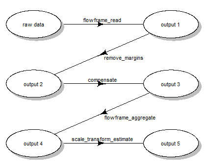
Scale transform processing queue
When this first part is done, one can apply pre-processing for each file one by one. However, depending on the choice of QC method, the order of steps needs to be slightly different:
- when using flowAI, it is advised to eliminate the ‘bad events’ starting from raw data (see (Monaco et al. 2016))
- when using PeacoQC, it is advised to eliminate the ‘bad events’ from already compensated and scale transformed data (see (Emmaneel et al. 2021))
Therefore, we propose the following pre-processing queues represented in Fig. 2.
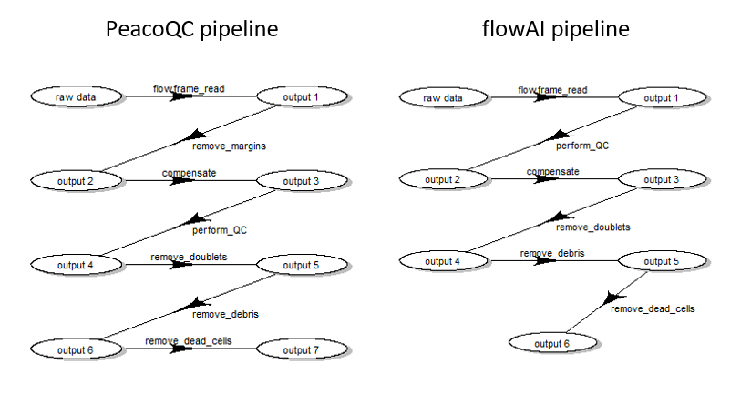
Pre-processing queue for two different pipeline settings
Building the CytoPipeline
CytoPipeline is the central S4 class used in the
CytoPipeline package to represent a flow cytometry
pre-processing pipeline. The main slots of CytoPipeline
objects are :
an
experimentName, which gives a name to a particular user definition of a pre-processing pipeline. The experiment here, is not related to an assay experiment, but refers to a specific way to design a pipeline. For example, in the current use case, we will define twoexperimentNames, one to refer to the flowAI pipeline, and another one to refer to the PeacoQC pipeline (see previous section);a vector of
sampleFiles, which are.fcsraw data files on which one need to run the pre-processing pipeline;two processing queues, i.e. a
scaleTransformProcessingQueue, and aflowFramesPreProcessingQueue, which correspond to the two parts described in previous section. Each of these queues are composed of one or severalCytoProcessingStepobjects, will be processed in linear sequence, the output of one step being the input of the next step.
Note there are important differences between the two processing
queues. On the one hand, the scaleTransformProcessingQueue
takes the vector of all sample files as an input, and will be executed
first, and only once. On the other hand, the
flowFramesPreProcessingQueue will be run after the scale
transformation processing queue, on each sample file one after the
other, within a loop. The final output of the
scaleTransformProcessingQueue, which should be a
flowCore::tranformList, is also provided as input to the
flowFramesPreProcessingQueue, by convention.
In the next subsections, we show the different steps involved in
creating a CytoPipeline object.
preliminaries: paths definition
In the following code, rawDataDir refers to the
directory in which the .fcs raw data files are stored.
workDir will be used as root directory to store the disk
cache. Indeed, when running the CytoPipeline objects, all
the different step outputs will be stored in a
BiocFileCache instance, in a sub-directory that will be
created in workDirand of which the name will be set to the
pipeline experimentName.
library(CytoPipeline)

# raw data
rawDataDir <- system.file("extdata", package = "CytoPipeline")
# output files
workDir <- suppressMessages(base::tempdir())
first method: step by step, using CytoPipeline methods
In this sub-section, we build a CytoPipeline object and
successively add CytoProcessingStep objects to the two
different processing queues. We do this for the PeacoQC pipeline.
# main parameters : sample files and output files

experimentName <- "OMIP021_PeacoQC"
sampleFiles <- file.path(rawDataDir, list.files(rawDataDir,
                                                pattern = "Donor"))

pipL_PeacoQC <- CytoPipeline(experimentName = experimentName,
                             sampleFiles = sampleFiles)

### SCALE TRANSFORMATION STEPS ###

pipL_PeacoQC <-
    addProcessingStep(pipL_PeacoQC,
        whichQueue = "scale transform",
        CytoProcessingStep(
            name = "flowframe_read",
            FUN = "readSampleFiles",
            ARGS = list(
                whichSamples = "all",
                truncate_max_range = FALSE,
                min.limit = NULL
            )
        )
    )

pipL_PeacoQC <-
    addProcessingStep(pipL_PeacoQC,
        whichQueue = "scale transform",
        CytoProcessingStep(
            name = "remove_margins",
            FUN = "removeMarginsPeacoQC",
            ARGS = list()
        )
    )

pipL_PeacoQC <-
    addProcessingStep(pipL_PeacoQC,
        whichQueue = "scale transform",
        CytoProcessingStep(
            name = "compensate",
            FUN = "compensateFromMatrix",
            ARGS = list(matrixSource = "fcs")
        )
    )

pipL_PeacoQC <-
    addProcessingStep(pipL_PeacoQC,
        whichQueue = "scale transform",
        CytoProcessingStep(
            name = "flowframe_aggregate",
            FUN = "aggregateAndSample",
            ARGS = list(
                nTotalEvents = 10000,
                seed = 0
            )
        )
    )

pipL_PeacoQC <-
    addProcessingStep(pipL_PeacoQC,
        whichQueue = "scale transform",
        CytoProcessingStep(
            name = "scale_transform_estimate",
            FUN = "estimateScaleTransforms",
            ARGS = list(
                fluoMethod = "estimateLogicle",
                scatterMethod = "linear",
                scatterRefMarker = "BV785 - CD3"
            )
        )
    )

### FLOW FRAME PRE-PROCESSING STEPS ###

pipL_PeacoQC <-
    addProcessingStep(pipL_PeacoQC,
        whichQueue = "pre-processing",
        CytoProcessingStep(
            name = "flowframe_read",
            FUN = "readSampleFiles",
            ARGS = list(
                truncate_max_range = FALSE,
                min.limit = NULL
            )
        )
    )


pipL_PeacoQC <-
    addProcessingStep(pipL_PeacoQC,
        whichQueue = "pre-processing",
        CytoProcessingStep(
            name = "remove_margins",
            FUN = "removeMarginsPeacoQC",
            ARGS = list()
        )
    )

pipL_PeacoQC <-
    addProcessingStep(pipL_PeacoQC,
        whichQueue = "pre-processing",
        CytoProcessingStep(
            name = "compensate",
            FUN = "compensateFromMatrix",
            ARGS = list(matrixSource = "fcs")
        )
    )

pipL_PeacoQC <-
    addProcessingStep(
        pipL_PeacoQC,
        whichQueue = "pre-processing",
        CytoProcessingStep(
            name = "perform_QC",
            FUN = "qualityControlPeacoQC",
            ARGS = list(
                preTransform = TRUE,
                min_cells = 150, # default
                max_bins = 500, # default
                step = 500, # default,
                MAD = 6, # default
                IT_limit = 0.55, # default
                force_IT = 150, # default
                peak_removal = 0.3333, # default
                min_nr_bins_peakdetection = 10 # default
            )
        )
    )

pipL_PeacoQC <-
    addProcessingStep(
        pipL_PeacoQC,
        whichQueue = "pre-processing",
        CytoProcessingStep(
            name = "remove_doublets",
            FUN = "removeDoubletsCytoPipeline",
            ARGS = list(
                areaChannels = c("FSC-A", "SSC-A"),
                heightChannels = c("FSC-H", "SSC-H"),
                nmads = c(3, 5))
            )
    )


pipL_PeacoQC <-
    addProcessingStep(pipL_PeacoQC,
        whichQueue = "pre-processing",
        CytoProcessingStep(
            name = "remove_debris",
            FUN = "removeDebrisManualGate",
            ARGS = list(
                FSCChannel = "FSC-A",
                SSCChannel = "SSC-A",
                gateData =  c(73615, 110174, 213000, 201000, 126000,
                              47679, 260500, 260500, 113000, 35000)
            )
        )
    )

pipL_PeacoQC <-
    addProcessingStep(pipL_PeacoQC,
        whichQueue = "pre-processing",
        CytoProcessingStep(
            name = "remove_dead_cells",
            FUN = "removeDeadCellsManualGate",
            ARGS = list(
                FSCChannel = "FSC-A",
                LDMarker = "L/D Aqua - Viability",
                gateData = c(0, 0, 250000, 250000,
                             0, 650, 650, 0)
            )
        )
    )
second method: in one go, using JSON file input
In this sub-section, we build the flowAI pipeline, this time using a
JSON file as an input. Note that the experimentName and
sampleFiles are here specified in the JSON file itself.
This is not necessary, as one could well specify the processing steps
only in the JSON file, and pass the experimentName and
sampleFiles directly in the CytoPipeline
constructor.
jsonDir <- rawDataDir

# creation on CytoPipeline object,
# using json file as input
pipL_flowAI <-
  CytoPipeline(file.path(jsonDir, "OMIP021_flowAI_pipeline.json"),
               experimentName = "OMIP021_flowAI",
               sampleFiles = sampleFiles)
Executing pipelines
Executing PeacoQC pipeline
Note: executing the next statement might generate some
warnings.
These are generated by the PeacoQC method, are highly
dependent on the shape of the data investigated, and can safely be
ignored here.
# execute PeacoQC pipeline
execute(pipL_PeacoQC, path = workDir)
## ####################################################### ### running SCALE TRANSFORMATION processing steps ##### ####################################################### Proceeding with step 1 [flowframe_read] ...## Proceeding with step 2 [remove_margins] ...## Removing margins from file : Donor1.fcs## Warning in PeacoQC::RemoveMargins(ff, channels = channel4Margins,
## channel_specifications = PQCChannelSpecs): More than 10.12 % is considered as a
## margin event in file Donor1.fcs . This should be verified.## Removing margins from file : Donor2.fcs## Proceeding with step 3 [compensate] ...## Proceeding with step 4 [flowframe_aggregate] ...## Warning in aggregateAndSample(new("flowSet", frames = <environment>, phenoData
## = new("AnnotatedDataFrame", : Could not choose as much as 10000 events for
## subsampling, sampled number of events = 9194## Proceeding with step 5 [scale_transform_estimate] ...## ####################################################### ### NOW PRE-PROCESSING FILE /__w/_temp/Library/CytoPipeline/extdata/Donor1.fcs...## ####################################################### Proceeding with step 1 [flowframe_read] ...## Proceeding with step 2 [remove_margins] ...## Removing margins from file : Donor1.fcs## Warning in PeacoQC::RemoveMargins(ff, channels = channel4Margins,
## channel_specifications = PQCChannelSpecs): More than 10.12 % is considered as a
## margin event in file Donor1.fcs . This should be verified.## Proceeding with step 3 [compensate] ...## Proceeding with step 4 [perform_QC] ...## Applying PeacoQC method...## Starting quality control analysis for Donor1.fcs## Warning in FindIncreasingDecreasingChannels(breaks, ff, channels, plot, : There
## seems to be an increasing or decreasing trend in a channel for Donor1.fcs .
## Please inspect this in the overview figure.## Calculating peaks## Warning in PeacoQC::PeacoQC(ff = ffIn, channels = channel4QualityControl, :
## There are not enough bins for a robust isolation tree analysis.## MAD analysis removed 38.81% of the measurements## The algorithm removed 38.81% of the measurements## Proceeding with step 5 [remove_doublets] ...## Proceeding with step 6 [remove_debris] ...## Proceeding with step 7 [remove_dead_cells] ...## ####################################################### ### NOW PRE-PROCESSING FILE /__w/_temp/Library/CytoPipeline/extdata/Donor2.fcs...## ####################################################### Proceeding with step 1 [flowframe_read] ...## Proceeding with step 2 [remove_margins] ...## Removing margins from file : Donor2.fcs## Proceeding with step 3 [compensate] ...## Proceeding with step 4 [perform_QC] ...## Applying PeacoQC method...## Starting quality control analysis for Donor2.fcs## Warning in FindIncreasingDecreasingChannels(breaks, ff, channels, plot, : There
## seems to be an increasing or decreasing trend in a channel for Donor2.fcs .
## Please inspect this in the overview figure.## Calculating peaks## Warning in PeacoQC::PeacoQC(ff = ffIn, channels = channel4QualityControl, :
## There are not enough bins for a robust isolation tree analysis.## MAD analysis removed 9.57% of the measurements## The algorithm removed 9.57% of the measurements## Proceeding with step 5 [remove_doublets] ...## Proceeding with step 6 [remove_debris] ...## Proceeding with step 7 [remove_dead_cells] ...Executing flowAI pipeline
Note: again this might generate some warnings, due to flowAI.
These are highly dependent on the shape of the data investigated, and
can safely be ignored here.
# execute flowAI pipeline
execute(pipL_flowAI, path = workDir)
## ####################################################### ### running SCALE TRANSFORMATION processing steps ##### ####################################################### Proceeding with step 1 [flowframe_read] ...## Proceeding with step 2 [remove_margins] ...## Removing margins from file : Donor1.fcs## Warning in PeacoQC::RemoveMargins(ff, channels = channel4Margins,
## channel_specifications = PQCChannelSpecs): More than 10.12 % is considered as a
## margin event in file Donor1.fcs . This should be verified.## Removing margins from file : Donor2.fcs## Proceeding with step 3 [compensate] ...## Proceeding with step 4 [flowframe_aggregate] ...## Warning in aggregateAndSample(new("flowSet", frames = <environment>, phenoData
## = new("AnnotatedDataFrame", : Could not choose as much as 10000 events for
## subsampling, sampled number of events = 9194## Proceeding with step 5 [scale_transform_estimate] ...## ####################################################### ### NOW PRE-PROCESSING FILE /__w/_temp/Library/CytoPipeline/extdata/Donor1.fcs...## ####################################################### Proceeding with step 1 [flowframe_read] ...## Proceeding with step 2 [perform_QC] ...## Applying flowAI method...## Quality control for the file: Donor1
## 5.46% of anomalous cells detected in the flow rate check.
## 0% of anomalous cells detected in signal acquisition check.
## 0.12% of anomalous cells detected in the dynamic range check.## Proceeding with step 3 [compensate] ...## Proceeding with step 4 [remove_doublets] ...## Proceeding with step 5 [remove_debris] ...## Proceeding with step 6 [remove_dead_cells] ...## ####################################################### ### NOW PRE-PROCESSING FILE /__w/_temp/Library/CytoPipeline/extdata/Donor2.fcs...## ####################################################### Proceeding with step 1 [flowframe_read] ...## Proceeding with step 2 [perform_QC] ...## Applying flowAI method...## Quality control for the file: Donor2
## 66.42% of anomalous cells detected in the flow rate check.
## 0% of anomalous cells detected in signal acquisition check.
## 0.1% of anomalous cells detected in the dynamic range check.## Proceeding with step 3 [compensate] ...## Proceeding with step 4 [remove_doublets] ...## Proceeding with step 5 [remove_debris] ...## Proceeding with step 6 [remove_dead_cells] ...Inspecting results and visualization
Plotting processing queues as workflow graphs
# plot work flow graph - PeacoQC - scale transformList
plotCytoPipelineProcessingQueue(
  pipL_PeacoQC,
  whichQueue = "scale transform",
  path = workDir)
PeacoQC pipeline - scale transformList processing queue
# plot work flow graph - PeacoQC - pre-processing
plotCytoPipelineProcessingQueue(
  pipL_PeacoQC,
  whichQueue = "pre-processing",
  sampleFile = 1,
  path = workDir)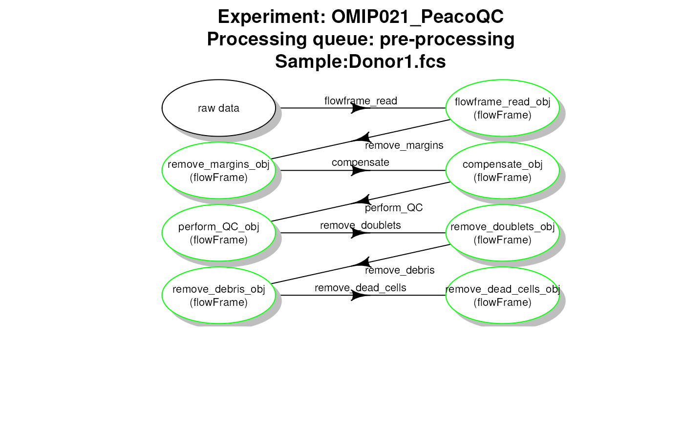
PeacoQC pipeline - file pre-processing queue
# plot work flow graph - flowAI - scale transformList
plotCytoPipelineProcessingQueue(
  pipL_flowAI,
  whichQueue = "scale transform",
  path = workDir)
flowAI pipeline - scale transformList processing queue
# plot work flow graph - flowAI - pre-processing

plotCytoPipelineProcessingQueue(
  pipL_flowAI,
  whichQueue = "pre-processing",
  sampleFile = 1,
  path = workDir)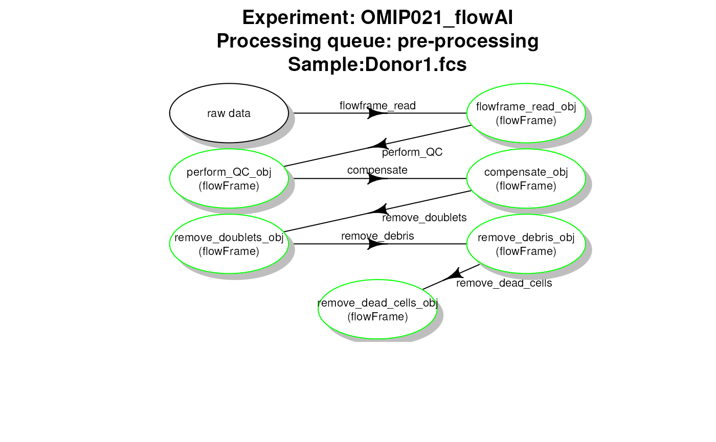
flowAI pipeline - file pre-processing queue
Obtaining information about pipeline generated objects
getCytoPipelineObjectInfos(pipL_PeacoQC,
                           path = workDir,
                           whichQueue = "scale transform")
## ObjectName ObjectClass
## 1 flowframe_read_obj flowSet
## 2 remove_margins_obj flowSet
## 3 compensate_obj flowSet
## 4 flowframe_aggregate_obj flowFrame
## 5 scale_transform_estimate_obj transformList
getCytoPipelineObjectInfos(pipL_PeacoQC,
                           path = workDir,
                           whichQueue = "pre-processing",
                           sampleFile = sampleFiles(pipL_PeacoQC)[1])
## ObjectName ObjectClass
## 1 flowframe_read_obj flowFrame
## 2 remove_margins_obj flowFrame
## 3 compensate_obj flowFrame
## 4 perform_QC_obj flowFrame
## 5 remove_doublets_obj flowFrame
## 6 remove_debris_obj flowFrame
## 7 remove_dead_cells_obj flowFrameRetrieving flow frames at different steps and plotting them
# example of retrieving a flow frame
# at a given step
ff <- getCytoPipelineFlowFrame(
  pipL_PeacoQC,
  whichQueue = "pre-processing",
  sampleFile = 1,
  objectName = "remove_doublets_obj",
  path = workDir)

#
ff2 <- getCytoPipelineFlowFrame(
  pipL_PeacoQC,
  whichQueue = "pre-processing",
  sampleFile = 1,
  objectName = "remove_debris_obj",
  path = workDir)
ggplotEvents(ff, xChannel = "FSC-A")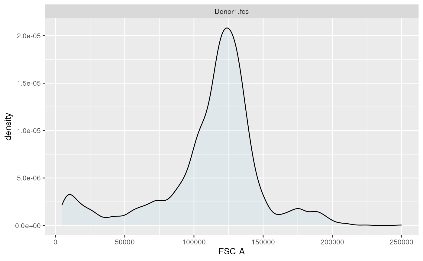
1-dimensional distribution plot (forward scatter channel)
ggplotEvents(ff, xChannel = "FSC-A", yChannel = "SSC-A")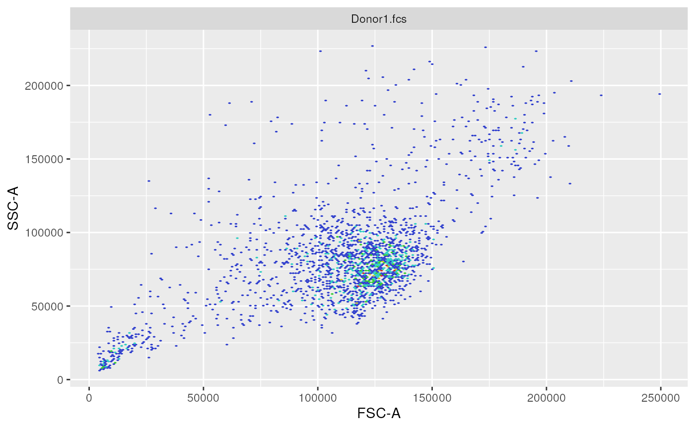
2-dimensional distribution plot (forward scatter vs. side scatter channels)
ggplotFilterEvents(ff, ff2, xChannel = "FSC-A", yChannel = "SSC-A")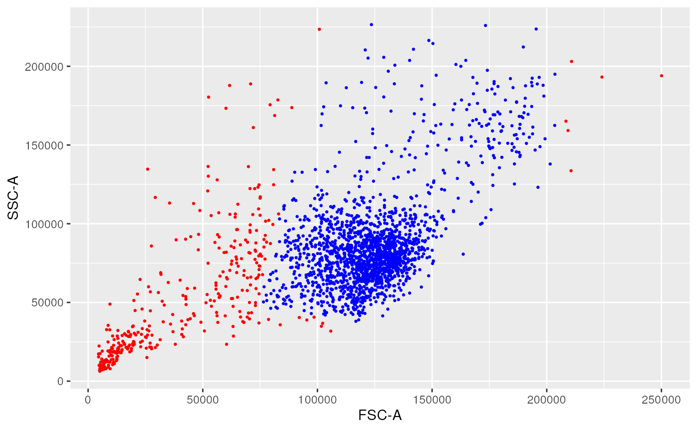
2-dimensional difference plot between remove_doublets and remove_debris steps
Example of retrieving another type of object
We now provide an example on how to retrieve an object from the
cache, that is not specifically a flowCore::flowFrame.
Here we retrieve a flowCore::flowSet object, which
represents a set offlowCore::flowFrameobjects, that was obtained after the
compensation step of the scale transformation processing queue, prior to
aggregating the two samples.
obj <- getCytoPipelineObjectFromCache(pipL_PeacoQC,
                                      path = workDir,
                                      whichQueue = "scale transform",
                                      objectName = "compensate_obj")
show(obj)
## A flowSet with 2 experiments.
##
## column names(22): FSC-A FSC-H ... Time Original_IDGetting and plotting the nb of retained events are each step
Getting the number of retained events at each pre-processing step, and tracking these changes throughout the pre-processing steps of a pipeline for different samples is a useful quality control.
This can be implemented using CytoPipeline
collectNbOfRetainedEvents() function. Examples of using
this function in quality control plots are shown in this section.
ret <- CytoPipeline::collectNbOfRetainedEvents(
    experimentName = "OMIP021_PeacoQC",
    path = workDir
)
ret
## flowframe_read remove_margins compensate perform_QC remove_doublets
## Donor1.fcs 5000 4494 4494 2750 2189
## Donor2.fcs 5000 4700 4700 4250 3431
## remove_debris remove_dead_cells
## Donor1.fcs 1850 1784
## Donor2.fcs 3019 2984
retainedProp <-
    as.data.frame(t(apply(
        ret,
        MARGIN = 1,
        FUN = function(line) {
            if (length(line) == 0 || is.na(line[1])) {
                as.numeric(rep(NA, length(line)))
            } else {
                round(line/line[1], 3)
            }
        }
    )))

retainedProp <- retainedProp[-1]

retainedProp
## remove_margins compensate perform_QC remove_doublets remove_debris
## Donor1.fcs 0.899 0.899 0.55 0.438 0.370
## Donor2.fcs 0.940 0.940 0.85 0.686 0.604
## remove_dead_cells
## Donor1.fcs 0.357
## Donor2.fcs 0.597
stepRemovedProp <-
    as.data.frame(t(apply(
        ret,
        MARGIN = 1,
        FUN = function(line) {
            if (length(line) == 0) {
                as.numeric(rep(NA, length(line)))
            } else {
                round(1-line/dplyr::lag(line), 3)
            }
        }
    )))

stepRemovedProp <- stepRemovedProp[-1]

stepRemovedProp
## remove_margins compensate perform_QC remove_doublets remove_debris
## Donor1.fcs 0.101 0 0.388 0.204 0.155
## Donor2.fcs 0.060 0 0.096 0.193 0.120
## remove_dead_cells
## Donor1.fcs 0.036
## Donor2.fcs 0.012
myGGPlot <- function(DF, title){
    stepNames = colnames(DF)
    rowNames = rownames(DF)
    DFLongFmt <- reshape(DF,
                         direction = "long",
                         v.names = "proportion",
                         varying = stepNames,
                         timevar = "step",
                         time = stepNames,
                         ids = rowNames)

    DFLongFmt$step <- factor(DFLongFmt$step, levels = stepNames)


    ggplot(data = DFLongFmt,
                 mapping = aes(x = step, y = proportion, text = id)) +
        geom_point(col = "blue") +
        ggtitle(title) +
        theme(axis.text.x = element_text(angle = 90))

}

p1 <- myGGPlot(DF = retainedProp,
               title = "Retained event proportion at each step")
p1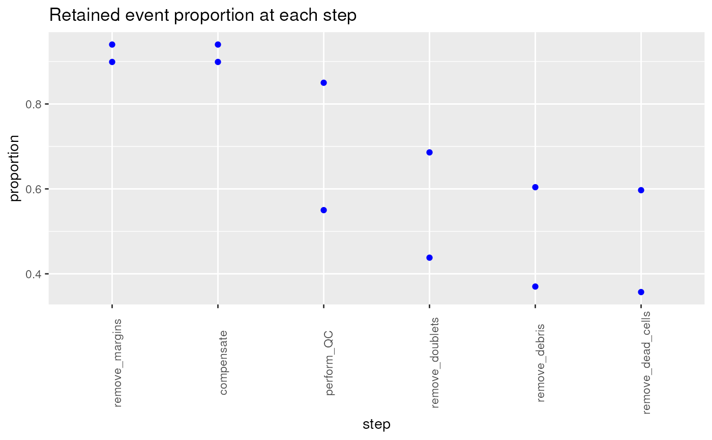
p2 <- myGGPlot(DF = stepRemovedProp,
               title = "Event proportion removed by each step")
p2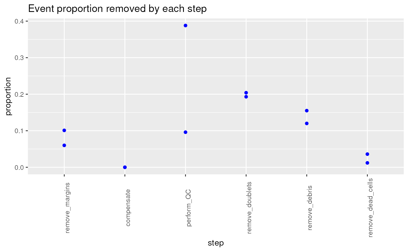
Interactive visualization
Using the CytoPipelineGUI package, it is possible to
interactively inspect results at the different steps of the pipeline,
either in the form of flowCore::flowFrame objects, or
flowCore::transformList. To do this, install the
CytoPipelineGUI package, and uncomment the following
code:
#devtools::install_github("https://github.com/UCLouvain-CBIO/CytoPipelineGUI")
#CytoPipelineGUI::CytoPipelineCheckApp(dir = workDir)
Adding function wrappers - note on the CytoPipelineUtils package
As was described in the previous sections, CytoPipeline
requires the user to provide wrappers to pre-processing functions, as
FUN parameter of CytoProcessingSteps. These
can be coded by the user themself, or come from a built-in function
provided in CytoPipeline itself.
However, in order to avoid having too many external dependencies for
CytoPipeline, another package
CytoPipelineUtils, is also available
CytoPipelineUtils is meant to be used in conjunction with
CytoPipeline package. It is a helper package, which is
aimed at hosting wrapper implementations of various functions of various
packages.
CytoPipelineUtils is open to contributions. If you want
to implement your own wrapper of your favourite pre-processing function
and use it in a CytoPipeline object, this is the place to
do it!
Session information
## R Under development (unstable) (2026-01-10 r89298)
## Platform: x86_64-pc-linux-gnu
## Running under: Ubuntu 24.04.3 LTS
##
## Matrix products: default
## BLAS:   /usr/lib/x86_64-linux-gnu/openblas-pthread/libblas.so.3
## LAPACK: /usr/lib/x86_64-linux-gnu/openblas-pthread/libopenblasp-r0.3.26.so;  LAPACK version 3.12.0
##
## locale:
##  [1] LC_CTYPE=en_US.UTF-8       LC_NUMERIC=C
##  [3] LC_TIME=en_US.UTF-8        LC_COLLATE=en_US.UTF-8
##  [5] LC_MONETARY=en_US.UTF-8    LC_MESSAGES=en_US.UTF-8
##  [7] LC_PAPER=en_US.UTF-8       LC_NAME=C
##  [9] LC_ADDRESS=C               LC_TELEPHONE=C
## [11] LC_MEASUREMENT=en_US.UTF-8 LC_IDENTIFICATION=C
##
## time zone: UTC
## tzcode source: system (glibc)
##
## attached base packages:
## [1] stats     graphics  grDevices utils     datasets  methods   base
##
## other attached packages:
## [1] ggplot2_4.0.1       reshape2_1.4.5      CytoPipeline_1.11.1
## [4] BiocStyle_2.39.0
##
## loaded via a namespace (and not attached):
##   [1] changepoint_2.3       tidyselect_1.2.1      dplyr_1.1.4
##   [4] farver_2.1.2          blob_1.3.0            filelock_1.0.3
##   [7] S7_0.2.1              fastmap_1.2.0         BiocFileCache_3.1.0
##  [10] XML_3.99-0.20         digest_0.6.39         lifecycle_1.0.5
##  [13] cluster_2.1.8.1       RSQLite_2.4.5         magrittr_2.0.4
##  [16] compiler_4.6.0        rlang_1.1.7           sass_0.4.10
##  [19] tools_4.6.0           yaml_2.3.12           data.table_1.18.0
##  [22] knitr_1.51            labeling_0.4.3        htmlwidgets_1.6.4
##  [25] bit_4.6.0             curl_7.0.0            diagram_1.6.5
##  [28] plyr_1.8.9            RColorBrewer_1.1-3    withr_3.0.2
##  [31] purrr_1.2.1           RProtoBufLib_2.23.0   BiocGenerics_0.57.0
##  [34] PeacoQC_1.21.0        desc_1.4.3            grid_4.6.0
##  [37] stats4_4.6.0          flowAI_1.41.0         colorspace_2.1-2
##  [40] scales_1.4.0          iterators_1.0.14      cli_3.6.5
##  [43] rmarkdown_2.30        crayon_1.5.3          ragg_1.5.0
##  [46] ncdfFlow_2.57.0       generics_0.1.4        otel_0.2.0
##  [49] rjson_0.2.23          DBI_1.2.3             cachem_1.1.0
##  [52] flowCore_2.23.1       stringr_1.6.0         parallel_4.6.0
##  [55] BiocManager_1.30.27   matrixStats_1.5.0     vctrs_0.6.5
##  [58] jsonlite_2.0.0        cytolib_2.23.0        bookdown_0.46
##  [61] IRanges_2.45.0        GetoptLong_1.1.0      S4Vectors_0.49.0
##  [64] bit64_4.6.0-1         clue_0.3-66           Rgraphviz_2.55.0
##  [67] systemfonts_1.3.1     foreach_1.5.2         jquerylib_0.1.4
##  [70] hexbin_1.28.5         glue_1.8.0            pkgdown_2.2.0.9000
##  [73] codetools_0.2-20      stringi_1.8.7         shape_1.4.6.1
##  [76] gtable_0.3.6          ggcyto_1.39.1         ComplexHeatmap_2.27.0
##  [79] tibble_3.3.1          pillar_1.11.1         rappdirs_0.3.3
##  [82] htmltools_0.5.9       graph_1.89.1          circlize_0.4.17
##  [85] R6_2.6.1              dbplyr_2.5.1          httr2_1.2.2
##  [88] textshaping_1.0.4     doParallel_1.0.17     evaluate_1.0.5
##  [91] flowWorkspace_4.23.1  lattice_0.22-7        Biobase_2.71.0
##  [94] png_0.1-8             memoise_2.0.1         bslib_0.9.0
##  [97] Rcpp_1.1.1            gridExtra_2.3         xfun_0.55
## [100] zoo_1.8-15            fs_1.6.6              pkgconfig_2.0.3
## [103] GlobalOptions_0.1.3