scplainer: reanalysis of the AML dataset (Schoof et al. 2021)

Introduction

In this vignette, we will analyse the schoof2021 dataset using the scplainer approach. The data were acquired using the SCoPE2-derived acquisition protocol (Schoof et al. 2021). Single cells were labelled with TMT-16 and MS data were acquired in DDA mode. The objective of the study was to show that mass spectrometry-based single-cell proteomics can effectively characterised the hierarchy of cellular differentiation in an accute myleoid leukemia model (AML).

Packages and data

We rely on several packages to compile this vignette.

## Core packages
library("scp")
library("scpdata")
library("SingleCellExperiment")
## Utility packages
library("ggplot2")
library("patchwork")
library("dplyr")
library("ensembldb")
library("EnsDb.Hsapiens.v86")
library("destiny")
library("scater")
library("plotly")

The data set is available from the scpdata package.

schoof <- schoof2021()
## see ?scpdata and browseVignettes('scpdata') for documentation
## loading from cache

The data set consists of four cell types as identied by upstream flow cytometry: leukemic stem cells (LSC), progenitor cells (PROG), CD38 positive blast cells (BLAST CD38+) and CD38 negative blast cells (BLAST CD38-).

table(schoof$Population)
## 
## BLAST CD38- BLAST CD38+         LSC        PROG 
##        1747         589          93          19

The dataset contains booster samples (also called carrier samples), empty wells, negative control samples, normalisation samples and single cells.

table(schoof$SampleType)
## 
## booster_1:1:1  booster_bulk         empty   neg control          norm 
##            72           120           192            48           192 
##            sc 
##          2448

The data were acquired using TMT-16 labelling.

table(schoof$Channel)
## 
##  126 127N 127C 128N 128C 129N 129C 130N 130C 131N 131C 132N 132C 133N 133C 134N 
##  192  192  192  192  192  192  192  192  192  192  192  192  192  192  192  192

The data were acquired as part of 192 MS acquisition batches.

length(levels(schoof$File.ID))
## [1] 192

Finally, samples were prepared through 8 sample preparation batches performed in 384-well plates.

table(schoof$Plate)
## 
##   bulk_b_1   bulk_b_2   bulk_b_3 bulk_b_e_1 bulk_b_e_2   bulk_c_1   bulk_c_2 
##        384        384        384        384        384        384        384 
##   bulk_c_3 
##        384

Minimal data processing

The minimal data processing workflow in scplainer consists of 5 main steps:

Data cleaning
Feature quality control
Sample quality control
Peptide data assembly
Log2-transformation

Cleaning data

We remove the protein assays that were processed by the authors. The vignette only uses the PTM data generated by Proteome Discoverer.

schoof <- removeAssay(schoof, c("proteins", "logNormProteins"))
## Warning: 'experiments' dropped; see 'drops()'
## harmonizing input:
##   removing 5097 sampleMap rows not in names(experiments)

We remove feature annotations that won’t be used in the remainder of the vignette. This is to avoid overcrowding of the annotation tables later in the vignette.

requiredRowData <- c(
    "Annotated.Sequence", "isContaminant",
    "Master.Protein.Accessions", "Isolation.Interference.in.Percent",
    "Percolator.q.Value"
)
schoof <- selectRowData(schoof, requiredRowData)

We replace zeros by missing values. A zero may be a true (the feature is not present in the sample) or because of technical limitations (due to the technology or the computational pre-processing). Because we are not able to distinguish between the two, zeros should be replaced with NA.

schoof <- zeroIsNA(schoof, i = names(schoof))

Feature quality control

We remove low-quality PSMs that may propagate technical artefacts and bias data modelling. The quality control criteria are:

We remove contaminants and decoy peptides.
We remove PSMs with low spectral purity.
We remove low-confidence peptides, as defined by the false discovery rate (FDR) computed by Percolator.
We remove PSMs for which the signal in single-cell samples exceeds 5% of the signal in 100-cell samples, i.e. the carrier.

All the criteria were readily computed except for the sample-to-carrier ratio. We compute this using computeSCR(). The results are stored in the rowData.

schoof <- computeSCR(
    schoof, names(schoof), colvar = "SampleType",
    samplePattern = "sc", carrierPattern = "^boost",
    sampleFUN = "mean", rowDataName = "MeanSCR"
)

Here is an overview of the distributions of each criteria

## `stat_bin()` using `bins = 30`. Pick better value with `binwidth`.
## `stat_bin()` using `bins = 30`. Pick better value with `binwidth`.
## `stat_bin()` using `bins = 30`. Pick better value with `binwidth`.
## Warning: Removed 25437 rows containing non-finite values (`stat_bin()`).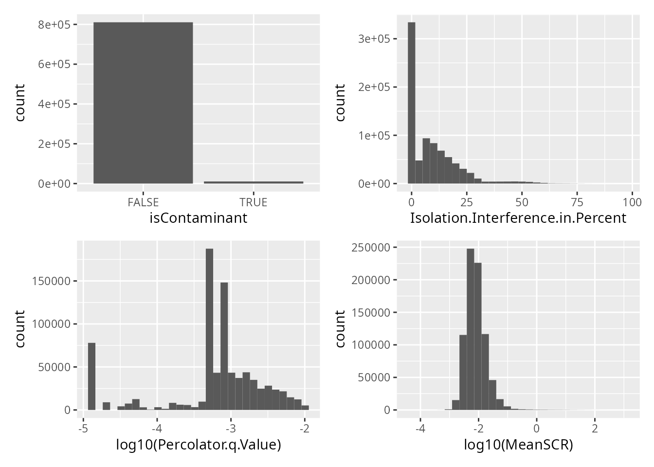

We filter and keep the features that pass the quality control criteria.

schoof <- filterFeatures(
    schoof, ~ Percolator.q.Value < 0.01 &
        !isContaminant & Master.Protein.Accessions != "" &
        Isolation.Interference.in.Percent < 30 &
        !is.na(MeanSCR) & MeanSCR < 0.2
)
## 'Percolator.q.Value' found in 192 out of 192 assay(s)
## 'isContaminant' found in 192 out of 192 assay(s)
## 'Master.Protein.Accessions' found in 192 out of 192 assay(s)
## 'Isolation.Interference.in.Percent' found in 192 out of 192 assay(s)
## 'MeanSCR' found in 192 out of 192 assay(s)

Sample quality control

Similarly to the features, we also remove low-quality cells. The quality control criteria are:

We remove samples with a low number of detected peptides. The criterion is computed as follows:

schoof <- countUniqueFeatures(
    schoof, i = names(schoof), groupBy = "Annotated.Sequence",
    colDataName = "NumberPeptides"
)

We remove samples with low median intensity. The metric (note we will later use it for normalisation) is computed as follows:

MedianIntensity <- lapply(experiments(schoof), function(x) {
    out <- colMedians(log(assay(x)), na.rm = TRUE)
    names(out) <- colnames(x)
    out
})
names(MedianIntensity) <- NULL
MedianIntensity <- unlist(MedianIntensity)
colData(schoof)[names(MedianIntensity), "MedianIntensity"] <- MedianIntensity

We remove the samples that have a high median coefficient of variation (CV). The CV is computed within each sample, by grouping the peptides that belong to the same protein or protein group. This is computed as follows:

schoof <- medianCVperCell(
    schoof, i = names(schoof), groupBy = "Master.Protein.Accessions",
    nobs = 3, na.rm = TRUE, colDataName = "MedianCV", norm = "SCoPE2"
)
## Warning in medianCVperCell(schoof, i = names(schoof), groupBy = "Master.Protein.Accessions", : The median CV could not be computed for one or more samples. You may want to try a smaller value for 'nobs'.

We also remove the samples that are not single cells because we will no longer need them.

We plot the metrics used to perform sample quality control.

ggplot(data.frame(colData(schoof))) +
    aes(
        y = MedianIntensity,
        x = NumberPeptides,
        color = MedianCV,
        shape = SampleType
    ) +
    geom_point(size = 2) +
    scale_color_continuous(type = "viridis")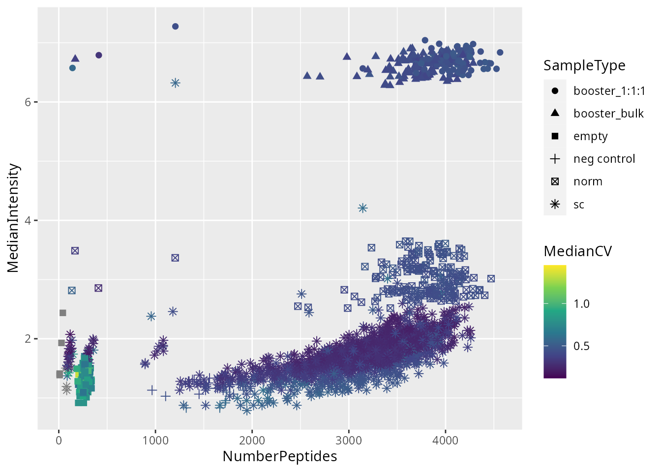

We apply the filter and keep only single cells that pass the quality control.

passQC <- !is.na(schoof$MedianCV) & schoof$MedianCV < 0.4 &
    schoof$MedianIntensity < 3 &
    schoof$NumberPeptides > 1200 &
    schoof$SampleType == "sc"
schoof <- subsetByColData(schoof, passQC)
schoof <- dropEmptyAssays(schoof)

Peptide data assembly

For now, each MS acquisition run is stored separately in an assay. We here combine these assays in one. The issue is that PSMs are specific to each run. We therefore aggregate the PSMs into peptides.

peptideAssays <- paste0("peptides_", names(schoof))
schoof <- aggregateFeatures(
    schoof,
    i = names(schoof),
    fcol = "Annotated.Sequence",
    name = peptideAssays,
    fun = colMedians,
    na.rm = TRUE
)

The data can now be joined.

schoof <- joinAssays(schoof, i = peptideAssays, name = "peptides")

Finally, we also convert Uniprot protein identifiers to gene symbols.

proteinIds <- rowData(schoof)[["peptides"]][, "Master.Protein.Accessions"]
## Unlist protein groups
proteinIds <- unlist(sapply(proteinIds, function(x) {
    strsplit(x, "; ")[[1]]
}, USE.NAMES = FALSE))
## Rename splice isoform number to canonical protein
proteinIds <- unique(sub("[-]\\d*$", "", proteinIds))
## Convert uniprot IDs to gene names
convert <- transcripts(
    EnsDb.Hsapiens.v86,
    columns = "gene_name",
    return.type = "data.frame",
    filter = UniprotFilter(proteinIds)
)
## Convert the protein groups into gene group
geneNames <- sapply(rowData(schoof)[["peptides"]]$Master.Protein.Accessions, function(x) {
        out <- strsplit(x, "; ")[[1]]
        out <- sapply(out, function(xx) {
            gene <- convert$gene_name[convert$uniprot_id == sub("[-]\\d*$", "", xx)]
            if (!length(gene)) return(NA)
            unique(gene)
        })
        paste(out, collapse = "; ")
    })
rowData(schoof)[["peptides"]]$Gene <- unname(geneNames)
head(rowData(schoof)[["peptides"]][, "Master.Protein.Accessions"])
## [1] "P05109"                 "P13639"                 "P60709; Q6S8J3; P68133"
## [4] "P19338"                 "P62249"                 "P29401"
head(rowData(schoof)[["peptides"]][, "Gene"])
## [1] "S100A8"             "EEF2"               "ACTB; POTEE; ACTA1"
## [4] "NCL"                "RPS16"              "TKT"

Log-transformation

We log2-transform the quantification data.

schoof <- logTransform(schoof, i = "peptides", name = "peptides_log")

Here is an overview of the data processing:

plot(schoof)
## Warning in plot.QFeatures(schoof): The QFeatures object contains many assays.
## You may want to consider creating an interactive plot (set 'interactive =
## TRUE')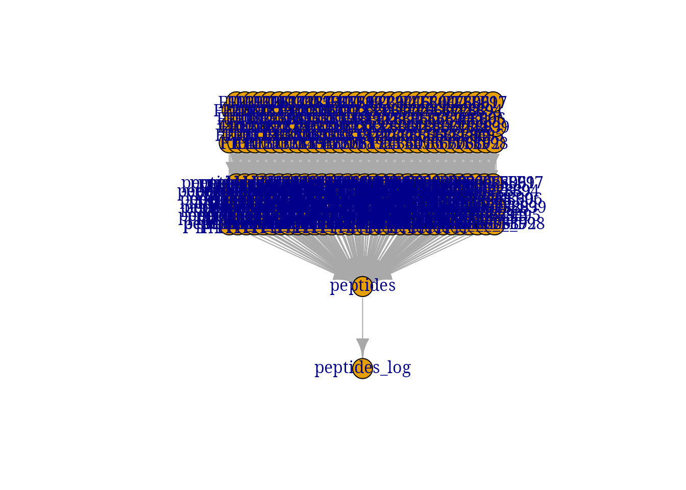

Data modelling

Model the data using scplainer, the linear regression model implemented in scp. scplainer is applied on a SingleCellExperiment so we extract it from the processed data set along with the colData

sce <- getWithColData(schoof, "peptides_log")

First, we must specify which variables to include in the model. We here include 4 variables:

MedianIntensity: this is the normalisation factor used to correct for cell-specific technical differences.
Channel: this is used to correct for TMT effects.
File.ID: this is used to perform batch correction. We consider each acquisition run to be a batch.
Population: this is the biological variable of interest. It captures the difference between the different AML populations

scpModelWorkflow() fits linear regression models to the data, where the model is adapted for each peptide depending on its pattern of missing values.

sce <- scpModelWorkflow(
    sce,
    formula = ~ 1 + ## intercept
        ## normalisation
        MedianIntensity +
        ## batch effects
        Channel + File.ID +
        ## biological variability
        Population
)

Once the models are fit, we can explore the distribution of the n/p ratios.

scpModelFilterThreshold(sce) <- 3
scpModelFilterPlot(sce)
## To change the threshold, use:
## scpModelFilterThreshold(object, name) <- threshold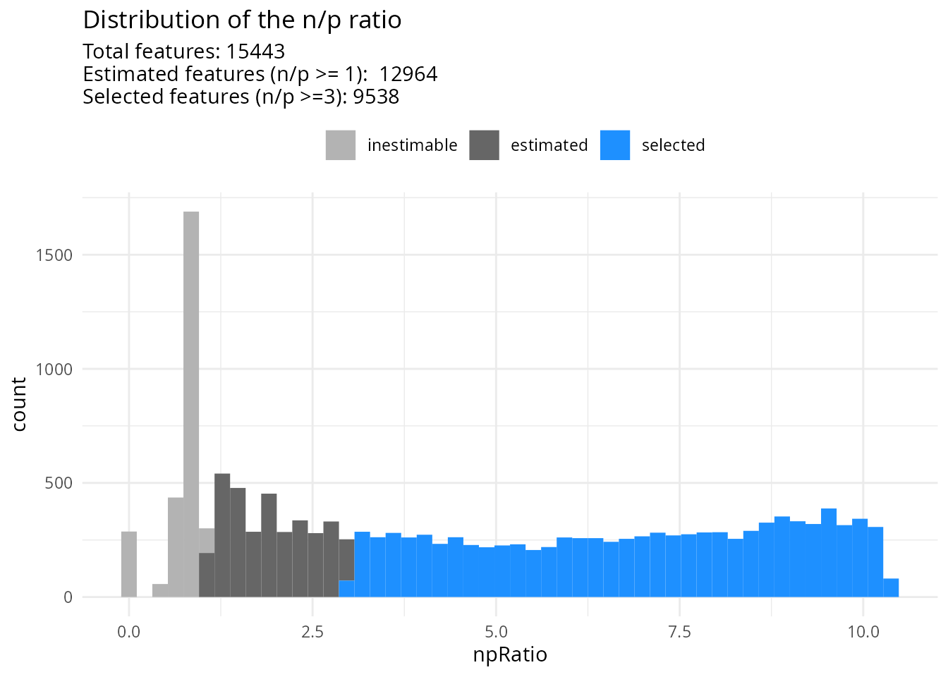

Many peptides do not have sufficient observations to estimate the model. We have chosen to continue the analysis with peptides that have \(n/p >= 3\). You could consider \(n/p\) a rough average of the number of replicates per parameter to fit (for categorical variables, the number of replicates per group). We recommend moving the threshold away from 1 to increase statistical power and remove noisy peptides. This comes of course at the cost of less peptides included in the analysis.

Model analysis

The model analysis consists of three steps:

Analysis of variance
Differential abundance analysis
Component analysis

Analysis of variance

The analysis of variance explores the proportion of data captures by each variable in the model.

(vaRes <- scpVarianceAnalysis(sce))
## DataFrameList of length 5
## names(5): Residuals MedianIntensity Channel File.ID Population
vaRes[[1]]
## DataFrame with 9538 rows and 4 columns
##            feature        SS        df percentExplainedVar
##        <character> <numeric> <numeric>           <numeric>
## 1    [-].mLTELE...  2578.954      1887             68.1597
## 2    [-].mVNFTV...   329.300      1889             22.1701
## 3    [K].aGFAGD...   519.815      1892             39.3162
## 4    [K].aLELTG...   554.172      1750             17.8839
## 5    [K].aLVAYY...   399.764      1624             22.4221
## ...            ...       ...       ...                 ...
## 9534 [R].eVQTAV...   45.2557       202             47.4447
## 9535 [R].iDEYDY...   52.8887       330             36.1397
## 9536 [R].tVVSGL...   29.9509       163             46.7577
## 9537 [K].aPQVVA...   15.3313        77             24.3418
## 9538 [K].aVTTPG...   27.0801        83             18.8546

The results are a list of tables, one table for each variable. Each table reports for each peptide the variance captures (SS), the residual degrees of freedom for estimating the variance (df) and the percentage of total variance explained (percentExplainedVar). To better explore the results, we add the annotations available in the rowData.

vaRes <- scpAnnotateResults(
    vaRes, rowData(sce), by = "feature", by2 = "Annotated.Sequence"
)

By default, we explore the variance for all peptides combined:

scpVariancePlot(vaRes)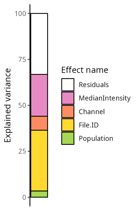

We explore the top 20 peptides that are have the highest percentage of variance explained by the biological variable (top) or by the batch variable (bottom).

scpVariancePlot(
    vaRes, top = 20, by = "percentExplainedVar", effect = "Population",
    decreasing = TRUE, combined = FALSE
) +
    scpVariancePlot(
    vaRes, top = 20, by = "percentExplainedVar", effect = "File.ID",
    decreasing = TRUE, combined = FALSE
) +
    plot_layout(ncol = 1, guides = "collect")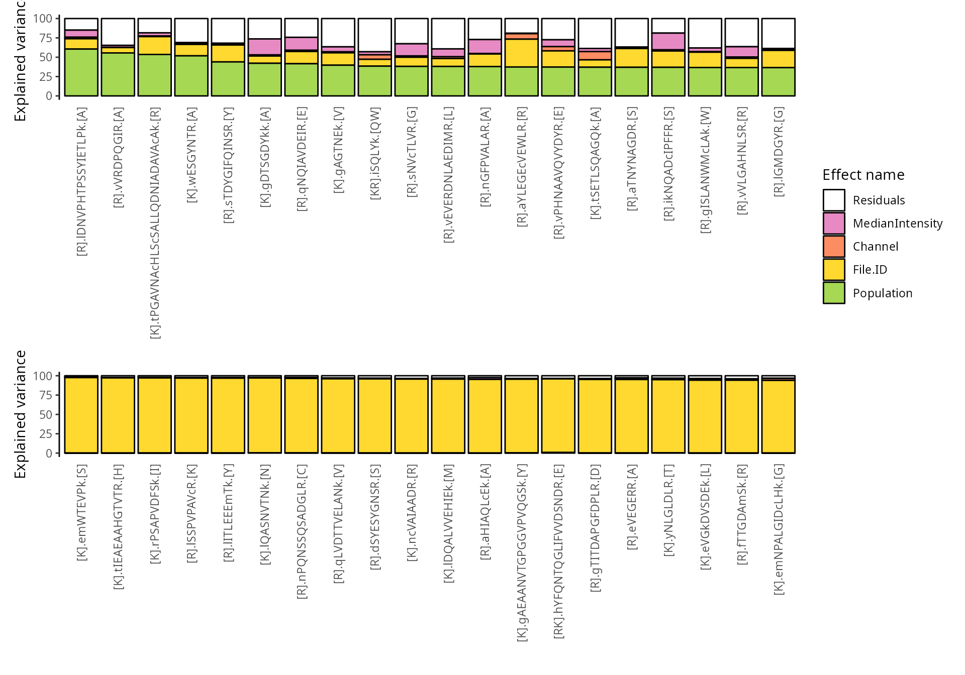

We can also group these peptide according to their protein. We simply need to provide the fcol argument.

scpVariancePlot(
    vaRes, top = 20, by = "percentExplainedVar", effect = "Population",
    decreasing = TRUE, combined = FALSE, fcol = "Gene"
) +
    scpVariancePlot(
    vaRes, top = 20, by = "percentExplainedVar", effect = "File.ID",
    decreasing = TRUE, combined = FALSE, fcol = "Gene"
) +
    plot_layout(ncol = 1, guides = "collect")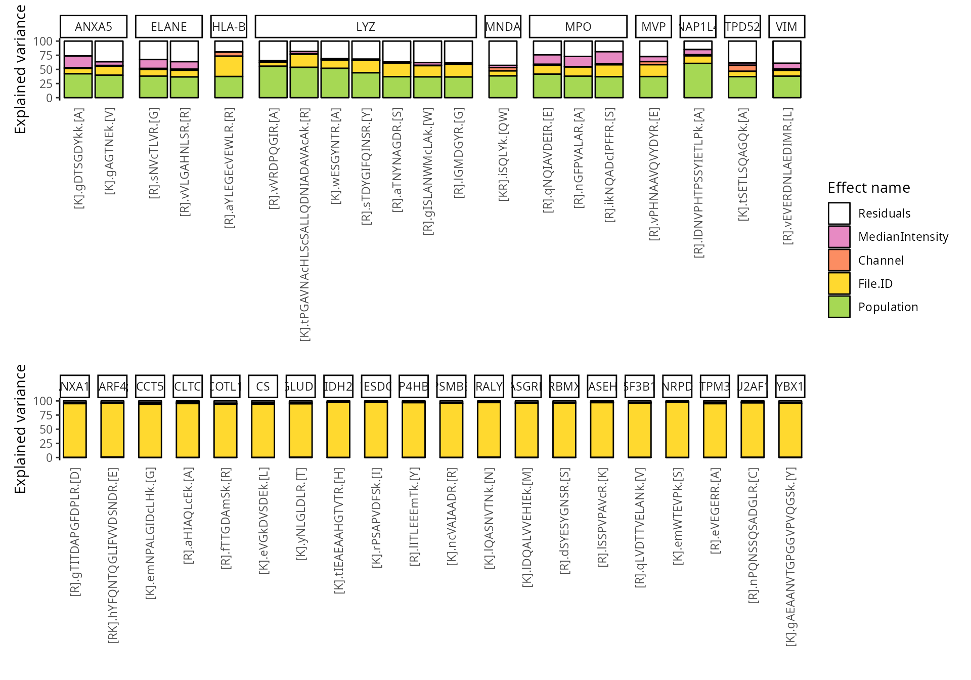

Differential abundance analysis

Next, we explore the model output to understand the differences between melanoma cells and monocytes. The difference of interest is specified using the contrast argument. The first element points to the variable to test and the two following element are the groups of interest to compare. You can provide multiple contrast in a list.

(daRes <- scpDifferentialAnalysis(
    sce, contrast = list(
        c("Population", "BLAST CD38-", "LSC"),
        c("Population", "BLAST CD38-", "PROG"),
        c("Population", "BLAST CD38-", "BLAST CD38+")
    )
))
## List of length 3
## names(3): Population_BLAST.CD38._vs_LSC ...
daRes[[1]]
## DataFrame with 9538 rows and 7 columns
##            feature   Estimate        SE        Df tstatistic      pvalue
##        <character>  <numeric> <numeric> <numeric>  <numeric>   <numeric>
## 1    [-].mLTELE...   0.872374 0.1674061      1887    5.21112 2.08235e-07
## 2    [-].mVNFTV...  -0.293451 0.0596068      1889   -4.92311 9.25829e-07
## 3    [K].aGFAGD...   0.242921 0.0748311      1892    3.24625 1.18980e-03
## 4    [K].aLELTG...  -0.658893 0.0807045      1750   -8.16426 6.11884e-16
## 5    [K].aLVAYY...  -0.268741 0.0734681      1624   -3.65792 2.62383e-04
## ...            ...        ...       ...       ...        ...         ...
## 9534 [R].eVQTAV... -0.1161121  0.145581       202 -0.7975772 0.426052446
## 9535 [R].iDEYDY... -0.3861179  0.111675       330 -3.4575012 0.000616609
## 9536 [R].tVVSGL... -0.4482902  0.206489       163 -2.1710103 0.031376758
## 9537 [K].aPQVVA...  0.0184523  0.205896        77  0.0896193 0.928822476
## 9538 [K].aVTTPG... -0.5251155  0.347445        83 -1.5113631 0.134494091
##             padj
##        <numeric>
## 1    4.48613e-06
## 2    1.72834e-05
## 3    8.88792e-03
## 4    5.53726e-14
## 5    2.47584e-03
## ...          ...
## 9534  0.70455105
## 9535  0.00508154
## 9536  0.12649213
## 9537  0.97715580
## 9538  0.35928109

Similarly to analysis of variance, the results are a list of tables, one table for each contrast. Each table reports for each peptide the estimated difference between the two groups, the standard error associated to the estimation, the degrees of freedom, the t-statistics, the associated p-value and the p-value FDR-adjusted for multiple testing across all peptides. Again, to better explore the results, we add the annotations available in the rowData.

daRes <- scpAnnotateResults(
    daRes, rowData(sce), 
    by = "feature", by2 = "Annotated.Sequence"
)

We then visualize the results using a volcano plot. The function below return a volcano plot for each contrast.

wrap_plots(scpVolcanoPlot(daRes))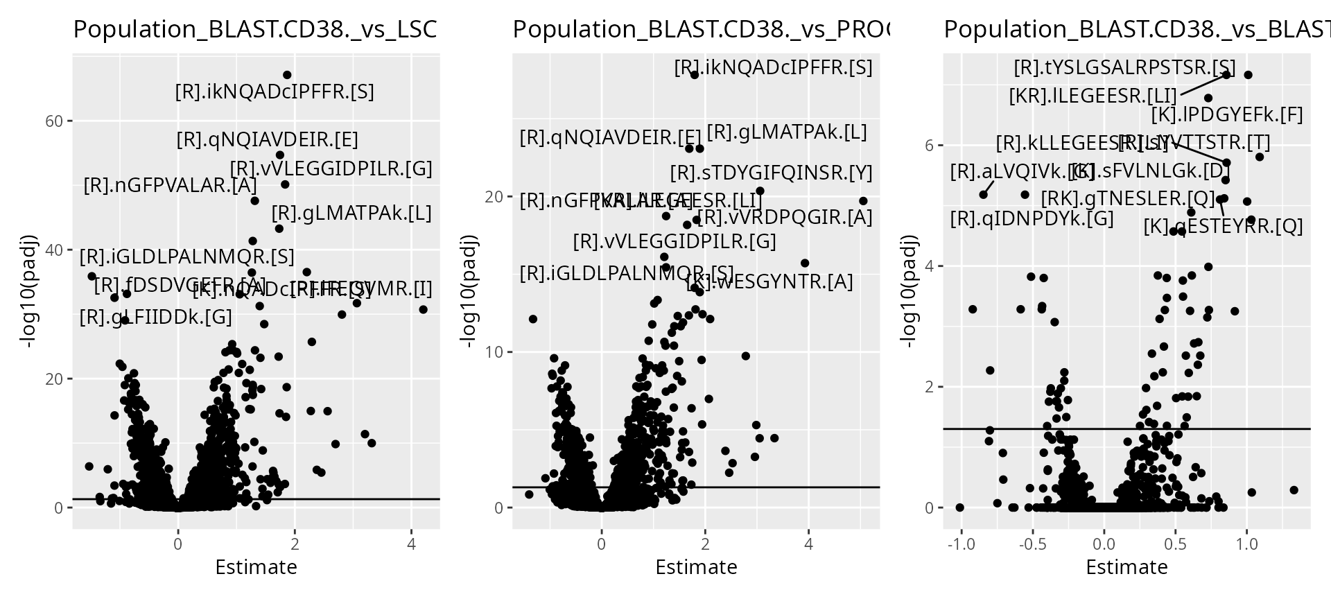

To help interpretation of the results, we will label the peptides with their gene name. Also we increase the number of labels shown on the plot. Finally, we can add colors to the plot. For instance, let’s explore the impact of the number of observations using the \(n/p\) ratio. We create a new annotation table, add it to the results and redraw the plot. The \(n/p\) ratio is retrieved using scpModelFilterNPRatio

np <- scpModelFilterNPRatio(sce)
daRes <- scpAnnotateResults(
    daRes, data.frame(feature = names(np), npRatio = np), 
    by = "feature"
)
wrap_plots(scpVolcanoPlot(
    daRes, top = 30, textBy = "Gene", 
    pointParams = list(aes(colour = npRatio))
))

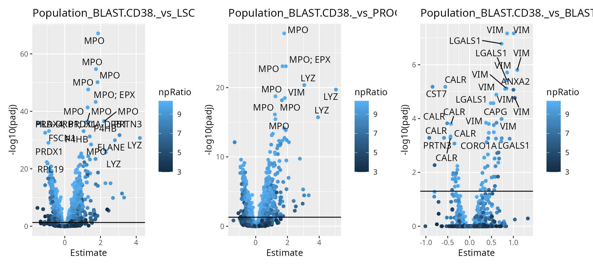
As expected, higher number of observations (higher \(n/p\)) lead to increased statistical power and hence to more significant results.

Finally, we offer functionality to report results at the protein level.

scpDifferentialAggregate(daRes, fcol = "Gene") |> 
    scpVolcanoPlot(top = 30) |> 
    wrap_plots()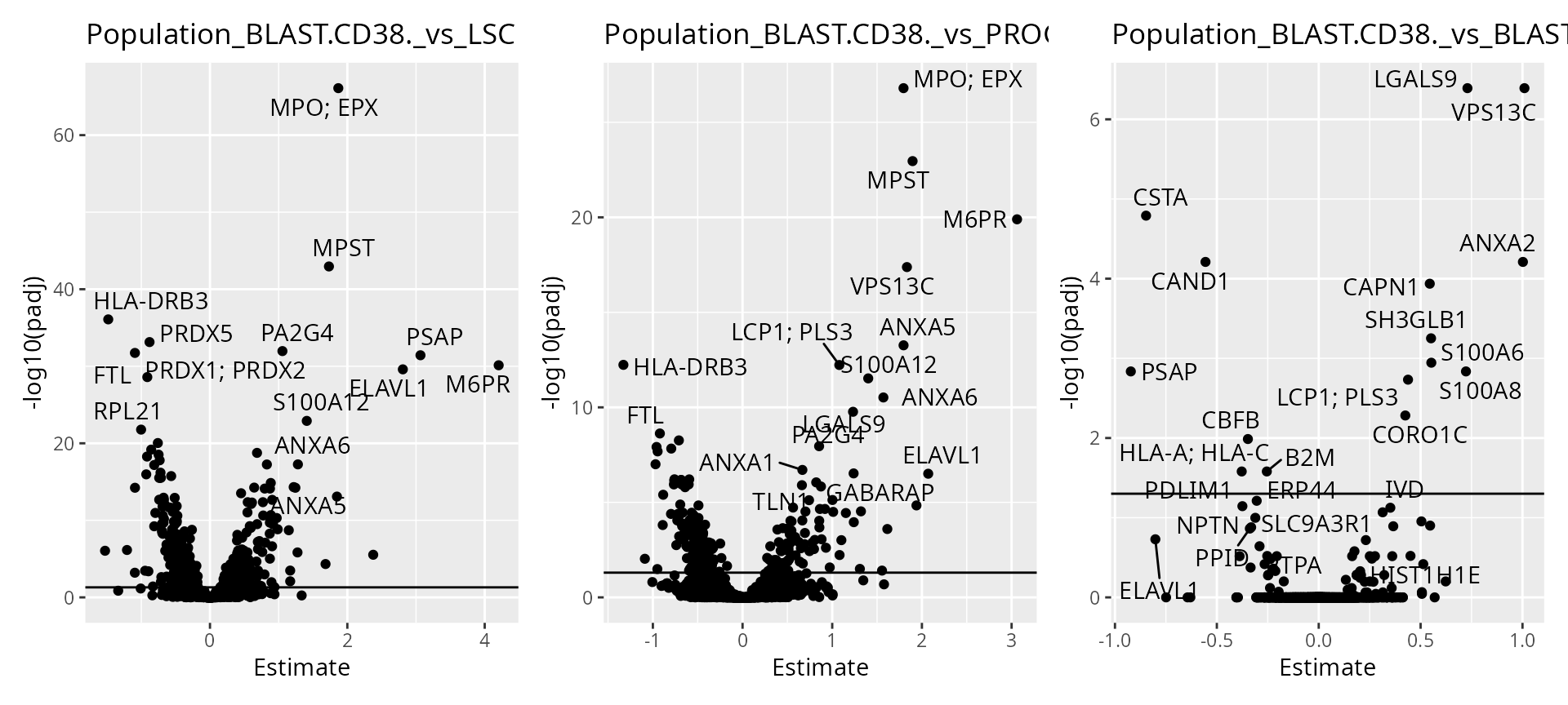

Component analysis

Finally, we perform component analysis to link the modelled effects to the cellular heterogeneity. We here run an APCA+ (extended ANOVA-simultaneous principal component analysis) for the sample type effect. In other words, we perform a PCA on the data that is capture by the sample type variable along with the residuals (unmodelled data).

(caRes <- scpComponentAnalysis(
    sce, ncomp = 2, method = "APCA", effect = "Population"
))
## [1] "APCA"
## [1] "Population"
## List of length 2
## names(2): bySample byFeature

The results are contained in a list with 2 elements. bySample contains the PC scores, that is the component results in sample space. byFeature contains the eigenvectors, that is the component results in feature space.

caRes$bySample
## List of length 3
## names(3): unmodelled residuals APCA_Population

Each of the two elements contains components results for the data before modelling (unmodelled), for the residuals or for the APCA on the sample type variable (APCA_Population).

caRes$bySample[[1]]
## DataFrame with 2118 rows and 3 columns
##                PC1       PC2        cell
##          <numeric> <numeric> <character>
## F1129N  -33.213784  -5.56117      F1129N
## F1129C   22.218813  -5.76867      F1129C
## F1130N    6.103797 -19.36936      F1130N
## F1130C  -13.577222  -5.21993      F1130C
## F1131N    0.991159  -5.26628      F1131N
## ...            ...       ...         ...
## F99132N   57.95420   8.32955     F99132N
## F99132C  -47.79824  -9.37227     F99132C
## F99133N   -6.75363 -12.73044     F99133N
## F99133C   31.14581  14.50989     F99133C
## F99134N  -15.61145  -3.46888     F99134N

Each elements is a table with the computed componoents. Let’s explore the component analysis results in cell space. Similarly to the previous explorations, we annotate the results.

caResCells <- caRes$bySample
sce$cell <- colnames(sce)
caResCells <- scpAnnotateResults(caResCells, colData(sce), by = "cell")

We then generate the component plot, colouring by Population.

scpComponentPlot(
    caResCells,
    pointParams = list(aes(colour = Population), alpha = 0.5)
) |>
    wrap_plots() +
    plot_layout(guides = "collect")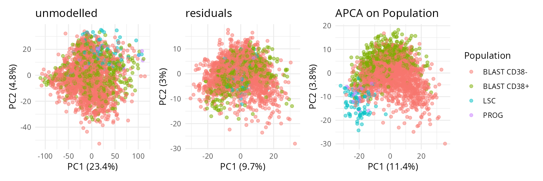

To assess the impact of batch effects, we shape the points according to the plate batch (cf intro) as well.

scpComponentPlot(
    caResCells,
    pointParams = list(aes(colour = as.numeric(File.ID)), alpha = 0.5)
) |>
    wrap_plots() +
    plot_layout(guides = "collect") &
    scale_color_continuous(type = "viridis")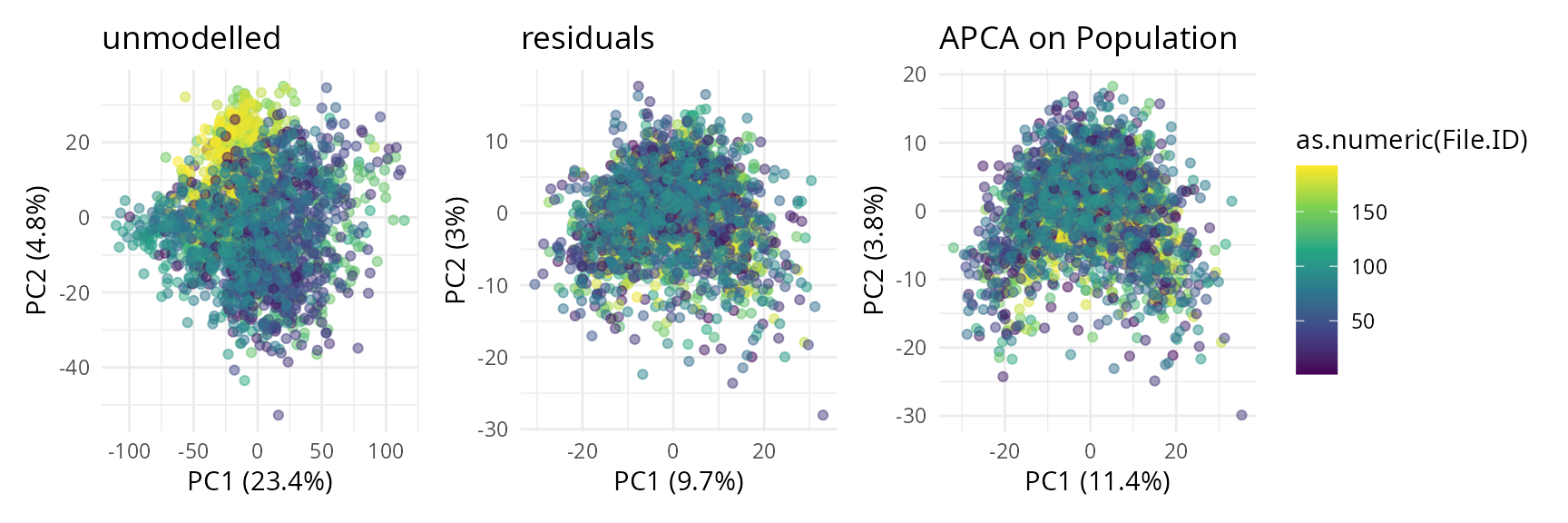

While the data before modelling is driven by batch effects with little biological effects, the APCA shows better separation of the four cell populations, with LSC progressively transitioning to PROG and then BLAST following the PC1 axis. However, strong residuals blurs the differences between populations, indicating that discretising the AML cell population into 4 populations may not be the most relevant approach for these data. We will explore this later during downstream analysis.

We use the same approach to explore the component results in feature space.

caResPeps <- caRes$byFeature
caResPeps <- scpAnnotateResults(
    caResPeps, rowData(sce), by = "feature", by2 = "Annotated.Sequence"
)

We plot the compenents in peptide-space.

plCApeps <- scpComponentPlot(
    caResPeps, pointParams = list(size = 0.8, alpha = 0.4)
)
wrap_plots(plCApeps)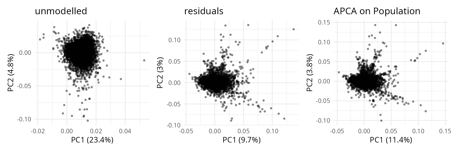

We can also combine the exploration of the components in cell and peptide space. This is possible thanks to biplots.

biplots <- scpComponentBiplot(
    caResCells, caResPeps, 
    pointParams = list(aes(colour = Population)),
    labelParams = list(size = 1.5, max.overlaps = 20),
    textBy = "Gene", top = 20
)
wrap_plots(biplots, guides = "collect")
## Warning: ggrepel: 14 unlabeled data points (too many overlaps). Consider
## increasing max.overlaps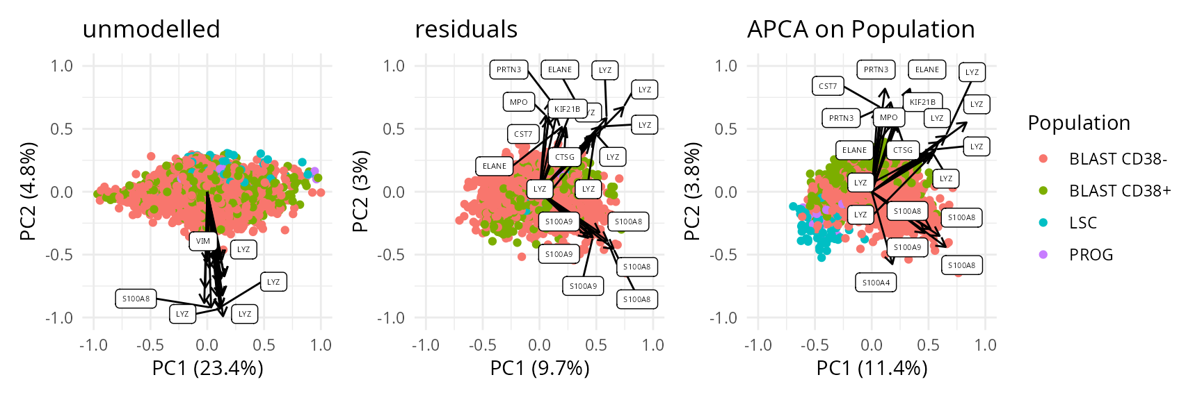

Finally, we offer functionality to aggregate the results at the protein level instead of the peptide level.

caResProts <- scpComponentAggregate(caResPeps, fcol = "Gene")
## Components may no longer be orthogonal after aggregation.
biplots <- scpComponentBiplot(
    caResCells, caResProts, 
    pointParams = list(aes(colour = Population)),
    labelParams = list(size = 1.5, max.overlaps = 20),
    textBy = "Gene", top = 20
)
wrap_plots(biplots, guides = "collect")
## Warning: ggrepel: 14 unlabeled data points (too many overlaps). Consider
## increasing max.overlaps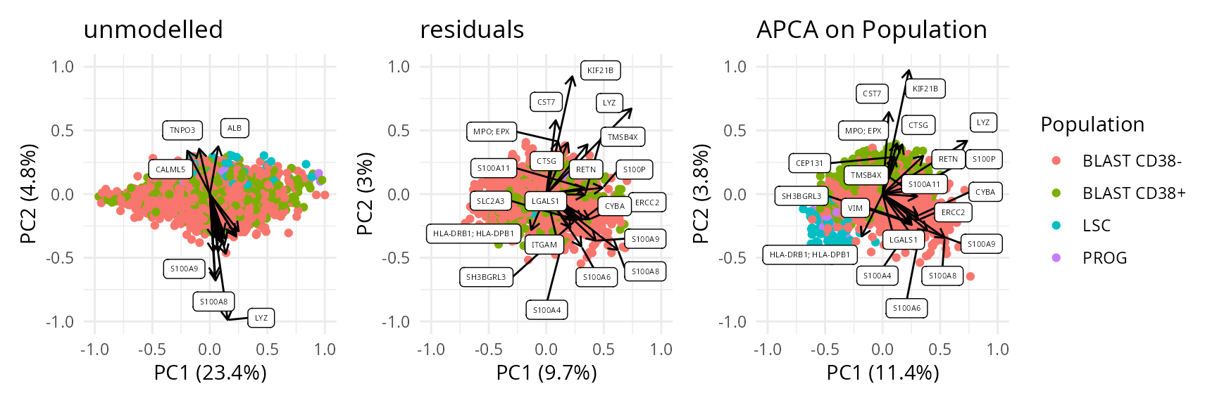

Interactive visualisation with iSEE

You can manually explore the data through an interactive interface thanks to iSEE:

library("iSEE")
iSEE(sce)

Downstream analysis

The final step in this analyses in the exploration of the differentiation trajectories of the AML model. To achieve this, we perform an APCA+ with more components to capture more of the variability. The APCA+ results are used to compute diffusion components that are used for diffusion pseudotime ordering.

Difusion pseudo-time analysis

We compute the 20 first APCA+ components on the sample type. We limit the PCA algorithm to 50 iterations to avoid an overly long run and will not compute the PCA for the unmodelled data and the residuals because we won’t use it during the downstream analysis.

apcaPopulation <- scpComponentAnalysis(
    sce, ncomp = 20, method = "APCA", effect = "Population", 
    residuals = FALSE, unmodelled = FALSE, maxiter = 50
)
## [1] "APCA"
## [1] "Population"
## Warning in nipals(t(mat), ncomp = ncomp, center = center, startcol = startcol, : Stopping after 50 iterations for PC 4.
## Warning in nipals(t(mat), ncomp = ncomp, center = center, startcol = startcol, : Stopping after 50 iterations for PC 6.
## Warning in nipals(t(mat), ncomp = ncomp, center = center, startcol = startcol, : Stopping after 50 iterations for PC 7.
## Warning in nipals(t(mat), ncomp = ncomp, center = center, startcol = startcol, : Stopping after 50 iterations for PC 8.
## Warning in nipals(t(mat), ncomp = ncomp, center = center, startcol = startcol, : Stopping after 50 iterations for PC 9.
## Warning in nipals(t(mat), ncomp = ncomp, center = center, startcol = startcol, : Stopping after 50 iterations for PC 10.
## Warning in nipals(t(mat), ncomp = ncomp, center = center, startcol = startcol, : Stopping after 50 iterations for PC 11.
## Warning in nipals(t(mat), ncomp = ncomp, center = center, startcol = startcol, : Stopping after 50 iterations for PC 12.
## Warning in nipals(t(mat), ncomp = ncomp, center = center, startcol = startcol, : Stopping after 50 iterations for PC 13.
## Warning in nipals(t(mat), ncomp = ncomp, center = center, startcol = startcol, : Stopping after 50 iterations for PC 14.
## Warning in nipals(t(mat), ncomp = ncomp, center = center, startcol = startcol, : Stopping after 50 iterations for PC 15.
## Warning in nipals(t(mat), ncomp = ncomp, center = center, startcol = startcol, : Stopping after 50 iterations for PC 16.
## Warning in nipals(t(mat), ncomp = ncomp, center = center, startcol = startcol, : Stopping after 50 iterations for PC 17.
## Warning in nipals(t(mat), ncomp = ncomp, center = center, startcol = startcol, : Stopping after 50 iterations for PC 18.
## Warning in nipals(t(mat), ncomp = ncomp, center = center, startcol = startcol, : Stopping after 50 iterations for PC 19.
## Warning in nipals(t(mat), ncomp = ncomp, center = center, startcol = startcol, : Stopping after 50 iterations for PC 20.
pca <- apcaPopulation$bySample$APCA_Population

The resulting components are stored in the SingleCellExperiment object.

pca <- as.matrix(pca[, grep("^PC", colnames(pca))])
reducedDim(sce, "APCA") <- pca

We compute the diffusion map from the PCA results.

dm <- DiffusionMap(pca)
## Warning: 'as(<dsCMatrix>, "dsTMatrix")' is deprecated.
## Use 'as(., "TsparseMatrix")' instead.
## See help("Deprecated") and help("Matrix-deprecated").
reducedDim(sce, "DiffusionMap") <- eigenvectors(dm)

Finally, we plot the three first diffusion components.

plot_ly(x = reducedDim(sce, "DiffusionMap")[, 1], 
        y = reducedDim(sce, "DiffusionMap")[, 2], 
        z = reducedDim(sce, "DiffusionMap")[, 3],
        color = sce$Population,
        type = "scatter3d",
        mode = "markers")

The diffusion map confirms the progressive transition from LSC to BLAST cells. However, we see an alternative differentiation track characterised by low scores for the second diffusion component.

Session information

R Under development (unstable) (2023-07-27 r84768)
Platform: x86_64-pc-linux-gnu
Running under: Ubuntu 23.04

Matrix products: default
BLAS:   /usr/lib/x86_64-linux-gnu/blas/libblas.so.3.11.0 
LAPACK: /usr/lib/x86_64-linux-gnu/lapack/liblapack.so.3.11.0

locale:
 [1] LC_CTYPE=en_US.UTF-8       LC_NUMERIC=C              
 [3] LC_TIME=en_US.UTF-8        LC_COLLATE=en_US.UTF-8    
 [5] LC_MONETARY=en_US.UTF-8    LC_MESSAGES=en_US.UTF-8   
 [7] LC_PAPER=en_US.UTF-8       LC_NAME=C                 
 [9] LC_ADDRESS=C               LC_TELEPHONE=C            
[11] LC_MEASUREMENT=en_US.UTF-8 LC_IDENTIFICATION=C       

time zone: Europe/Prague
tzcode source: system (glibc)

attached base packages:
[1] stats4    stats     graphics  grDevices utils     datasets  methods  
[8] base     

other attached packages:
 [1] plotly_4.10.3               scater_1.31.0              
 [3] scuttle_1.13.0              destiny_3.17.0             
 [5] EnsDb.Hsapiens.v86_2.99.0   ensembldb_2.27.0           
 [7] AnnotationFilter_1.27.0     GenomicFeatures_1.55.1     
 [9] AnnotationDbi_1.65.2        dplyr_1.1.3                
[11] patchwork_1.1.3             ggplot2_3.4.4              
[13] SingleCellExperiment_1.25.0 scpdata_1.9.2              
[15] ExperimentHub_2.11.0        AnnotationHub_3.11.0       
[17] BiocFileCache_2.11.1        dbplyr_2.4.0               
[19] scp_1.11.3                  QFeatures_1.13.0           
[21] MultiAssayExperiment_1.29.0 SummarizedExperiment_1.33.0
[23] Biobase_2.63.0              GenomicRanges_1.55.1       
[25] GenomeInfoDb_1.39.0         IRanges_2.37.0             
[27] S4Vectors_0.41.1            BiocGenerics_0.49.1        
[29] MatrixGenerics_1.15.0       matrixStats_1.1.0          
[31] BiocStyle_2.31.0           

loaded via a namespace (and not attached):
  [1] fs_1.6.3                      ProtGenerics_1.35.0          
  [3] bitops_1.0-7                  httr_1.4.7                   
  [5] RColorBrewer_1.1-3            tools_4.4.0                  
  [7] utf8_1.2.4                    R6_2.5.1                     
  [9] lazyeval_0.2.2                withr_2.5.2                  
 [11] sp_2.1-1                      prettyunits_1.2.0            
 [13] gridExtra_2.3                 fdrtool_1.2.17               
 [15] cli_3.6.1                     textshaping_0.3.7            
 [17] labeling_0.4.3                slam_0.1-50                  
 [19] nipals_0.8                    sass_0.4.7                   
 [21] robustbase_0.99-0             proxy_0.4-27                 
 [23] pkgdown_2.0.7                 Rsamtools_2.19.2             
 [25] systemfonts_1.0.5             TTR_0.24.3                   
 [27] rstudioapi_0.15.0             RSQLite_2.3.3                
 [29] generics_0.1.3                BiocIO_1.13.0                
 [31] crosstalk_1.2.0               car_3.1-2                    
 [33] Matrix_1.6-1.1                ggbeeswarm_0.7.2             
 [35] fansi_1.0.5                   abind_1.4-5                  
 [37] lifecycle_1.0.4               scatterplot3d_0.3-44         
 [39] yaml_2.3.7                    carData_3.0-5                
 [41] SparseArray_1.3.0             grid_4.4.0                   
 [43] blob_1.2.4                    promises_1.2.1               
 [45] crayon_1.5.2                  lattice_0.22-5               
 [47] beachmat_2.19.0               KEGGREST_1.43.0              
 [49] pillar_1.9.0                  knitr_1.45                   
 [51] metapod_1.11.0                rjson_0.2.21                 
 [53] boot_1.3-28.1                 codetools_0.2-19             
 [55] glue_1.6.2                    pcaMethods_1.95.0            
 [57] data.table_1.14.8             vcd_1.4-11                   
 [59] vctrs_0.6.4                   png_0.1-8                    
 [61] gtable_0.3.4                  cachem_1.0.8                 
 [63] xfun_0.41                     S4Arrays_1.3.0               
 [65] mime_0.12                     RcppEigen_0.3.3.9.4          
 [67] interactiveDisplayBase_1.41.0 ellipsis_0.3.2               
 [69] xts_0.13.1                    bit64_4.0.5                  
 [71] progress_1.2.2                filelock_1.0.2               
 [73] rprojroot_2.0.4               bslib_0.5.1                  
 [75] irlba_2.3.5.1                 vipor_0.4.5                  
 [77] colorspace_2.1-0              DBI_1.1.3                    
 [79] nnet_7.3-19                   tidyselect_1.2.0             
 [81] smoother_1.1                  bit_4.0.5                    
 [83] compiler_4.4.0                curl_5.1.0                   
 [85] BiocNeighbors_1.21.0          xml2_1.3.5                   
 [87] desc_1.4.2                    DelayedArray_0.29.0          
 [89] bookdown_0.36                 rtracklayer_1.63.0           
 [91] scales_1.2.1                  DEoptimR_1.1-3               
 [93] lmtest_0.9-40                 hexbin_1.28.3                
 [95] rappdirs_0.3.3                stringr_1.5.0                
 [97] digest_0.6.33                 rmarkdown_2.25               
 [99] XVector_0.43.0                htmltools_0.5.7              
[101] pkgconfig_2.0.3               sparseMatrixStats_1.15.0     
[103] lpsymphony_1.31.0             highr_0.10                   
[105] fastmap_1.1.1                 rlang_1.1.2                  
[107] htmlwidgets_1.6.2             ggthemes_4.2.4               
[109] shiny_1.7.5.1                 DelayedMatrixStats_1.25.0    
[111] farver_2.1.1                  jquerylib_0.1.4              
[113] IHW_1.31.0                    zoo_1.8-12                   
[115] jsonlite_1.8.7                BiocParallel_1.37.0          
[117] BiocSingular_1.19.0           RCurl_1.98-1.13              
[119] magrittr_2.0.3                GenomeInfoDbData_1.2.11      
[121] munsell_0.5.0                 Rcpp_1.0.11                  
[123] viridis_0.6.4                 MsCoreUtils_1.15.1           
[125] stringi_1.7.12                zlibbioc_1.49.0              
[127] MASS_7.3-60.1                 parallel_4.4.0               
[129] ggrepel_0.9.4                 Biostrings_2.71.1            
[131] hms_1.1.3                     igraph_1.5.1                 
[133] ranger_0.15.1                 RcppHNSW_0.5.0               
[135] biomaRt_2.59.0                ScaledMatrix_1.11.0          
[137] BiocVersion_3.19.1            XML_3.99-0.15                
[139] evaluate_0.23                 BiocManager_1.30.22          
[141] laeken_0.5.2                  httpuv_1.6.12                
[143] VIM_6.2.2                     tidyr_1.3.0                  
[145] purrr_1.0.2                   knn.covertree_1.0            
[147] clue_0.3-65                   BiocBaseUtils_1.5.0          
[149] rsvd_1.0.5                    xtable_1.8-4                 
[151] restfulr_0.0.15               e1071_1.7-13                 
[153] RSpectra_0.16-1               later_1.3.1                  
[155] viridisLite_0.4.2             class_7.3-22                 
[157] ragg_1.2.6                    tibble_3.2.1                 
[159] memoise_2.0.1                 beeswarm_0.4.0               
[161] GenomicAlignments_1.39.0      cluster_2.1.4                
[163] ggplot.multistats_1.0.0

Citation

citation("scp")
To cite the scp package in publications use:

  Vanderaa, Christophe, and Laurent Gatto. 2023.  Revisiting the Thorny
  Issue of Missing Values in Single-Cell Proteomics. Journal of
  Proteome Research 22 (9): 2775–84.

  Vanderaa Christophe and Laurent Gatto. The current state of
  single-cell proteomics data analysis. Current Protocols 3 (1): e658.;
  doi: https://doi.org/10.1002/cpz1.658 (2023).

  Vanderaa Christophe and Laurent Gatto. Replication of Single-Cell
  Proteomics Data Reveals Important Computational Challenges. Expert
  Review of Proteomics, 1–9 (2021).

To see these entries in BibTeX format, use 'print(<citation>,
bibtex=TRUE)', 'toBibtex(.)', or set
'options(citation.bibtex.max=999)'.

License

This vignette is distributed under a CC BY-SA license license.

christophe.vanderaa@uclouvain.be ↩︎

Christophe Vanderaa¹, Computational Biology, UCLouvain

Laurent Gatto, Computational Biology, UCLouvain

8 December 2023

Introduction

Packages and data

Minimal data processing

Cleaning data

Feature quality control

Sample quality control

Peptide data assembly

Log-transformation

Data modelling

Model analysis

Analysis of variance

Differential abundance analysis

Component analysis

Interactive visualisation with iSEE

Downstream analysis

Difusion pseudo-time analysis

Session information

Citation

License

scplainer: reanalysis of the AML dataset (Schoof et al. 2021)

Christophe Vanderaa1, Computational Biology, UCLouvain

Laurent Gatto, Computational Biology, UCLouvain

8 December 2023

Introduction

Packages and data

Minimal data processing

Cleaning data

Feature quality control

Sample quality control

Peptide data assembly

Log-transformation

Data modelling

Model analysis

Analysis of variance

Differential abundance analysis

Component analysis

Interactive visualisation with iSEE

Downstream analysis

Difusion pseudo-time analysis

Session information

Citation

License

Christophe Vanderaa¹, Computational Biology, UCLouvain