Chapter 5 Manipulating and analyzing data with dplyr
Learning Objectives
Describe the purpose of the
dplyrandtidyrpackages.Select certain columns in a data frame with the
dplyrfunctionselect.Select certain rows in a data frame according to filtering conditions with the
dplyrfunctionfilter.Link the output of one
dplyrfunction to the input of another function with the ‘pipe’ operator%>%or|>.Add new columns to a data frame that are functions of existing columns with
mutate.Use the split-apply-combine concept for data analysis.
Use
summarize,group_by, andcountto split a data frame into groups of observations, apply summary statistics for each group, and then combine the results.Describe the concept of a wide and a long table format and for which purpose those formats are useful.
Reshape a data frame from long to wide format and back with the
pivot_wider()andpivot_longer()commands from thetidyrpackage.
5.1 Data Manipulation using dplyr and tidyr
Bracket subsetting is handy, but it can be cumbersome and difficult to
read, especially for complicated operations. Enter
dplyr. dplyr is a package for making tabular data
manipulation easier. It pairs nicely with tidyr which enables
you to swiftly convert between different data formats for plotting and
analysis.
Packages in R are basically sets of additional functions that let you
do more stuff. The functions we’ve been using so far, like str() or
data.frame(), come built into R; packages give you access to more of
them. Before you use a package for the first time you need to install
it on your machine, and then you should import it in every subsequent
R session when you need it. You should already have installed the
tidyverse package. This is an “umbrella-package” that installs
several packages useful for data analysis which work together well
such as tidyr, dplyr, ggplot2, tibble, etc.
The tidyverse packages address 3
common issues that arise when doing data analysis with some of
functions that come with R:
- The results from a base R function sometimes depend on the type of data.
- Using R expressions in a non standard way, which can be confusing for new learners.
- Hidden arguments, having default operations that new learners are not aware of.
Let’s start by loading several of the tidyverse packages with:
The Data Transformation Cheat
Sheet
provides an overview of the dplyr grammar, offering more details and
functions that we will see in this chapter. The Tidy Data
Tutor is a wonderful tool to visually
describe what the tidy data operations do. The following
tutorial
offers nice animations of mutate(), summarize(), group_by(), and
ungroup().
5.2 What are dplyr and tidyr?
The package dplyr provides easy tools for the most common data
manipulation tasks. It is built to work directly with data frames,
with many common tasks optimized by being written in a compiled
language (C++). An additional feature is the ability to work directly
with data stored in an external database. The benefits of doing this
are that the data can be managed natively in a relational database,
queries can be conducted on that database, and only the results of the
query are returned.
This addresses a common problem with R in that all operations are conducted in-memory and thus the amount of data you can work with is limited by available memory. The database connections essentially remove that limitation in that you can connect to a database of many hundreds of GB, conduct queries on it directly, and pull back into R only what you need for analysis.
The package tidyr addresses the common problem of wanting to
reshape your data for plotting and use by different R
functions. Sometimes we want data sets where we have one row per
measurement. Sometimes we want a data frame where each measurement
type has its own column, and rows are instead more aggregated groups -
like plots or aquaria. Moving back and forth between these formats is
nontrivial, and tidyr gives you tools for this and more
sophisticated data manipulation.
To learn more about dplyr and tidyr after the workshop,
you may want to check out this handy data transformation with
dplyr
cheatsheet
and this one about
tidyr.
We’ll read in our data using the read_csv() function, from the
tidyverse package readr, instead of read.csv().
## Rows: 32428 Columns: 19
## ── Column specification ───────────────────────────────────────────────────────────────────────────────────────────────
## Delimiter: ","
## chr (14): gene, sample, organism, sex, infection, strain, tissue, product, e...
## dbl  (5): expression, age, time, mouse, ENTREZID
##
## ℹ Use `spec()` to retrieve the full column specification for this data.
## ℹ Specify the column types or set `show_col_types = FALSE` to quiet this message.Notice that the class of the data is now tbl_df
This is referred to as a “tibble”. Tibbles tweak some of the behaviors of the data frame objects we introduced in the previous episode. The data structure is very similar to a data frame. For our purposes the only differences are that:
- In addition to displaying the data type of each column under its name, it only prints the first few rows of data and only as many columns as fit on one screen.
- Columns of class
characterare never converted into factors.
We’re going to learn some of the most common dplyr functions:
-
select(): subset columns -
filter(): subset rows on conditions -
mutate(): create new columns by using information from other columns -
group_by()andsummarize(): create summary statisitcs on grouped data -
arrange(): sort results -
count(): count discrete values
5.3 Selecting columns and filtering rows
To select columns of a data frame, use select(). The first argument
to this function is the data frame (rna), and the subsequent
arguments are the columns to keep.
## # A tibble: 32,428 × 4
##    gene    sample     tissue     expression
##    <chr>   <chr>      <chr>           <dbl>
##  1 Asl     GSM2545336 Cerebellum       1170
##  2 Apod    GSM2545336 Cerebellum      36194
##  3 Cyp2d22 GSM2545336 Cerebellum       4060
##  4 Klk6    GSM2545336 Cerebellum        287
##  5 Fcrls   GSM2545336 Cerebellum         85
##  6 Slc2a4  GSM2545336 Cerebellum        782
##  7 Exd2    GSM2545336 Cerebellum       1619
##  8 Gjc2    GSM2545336 Cerebellum        288
##  9 Plp1    GSM2545336 Cerebellum      43217
## 10 Gnb4    GSM2545336 Cerebellum       1071
## # ℹ 32,418 more rows
To select all columns except certain ones, put a “-” in front of the variable to exclude it.
## # A tibble: 32,428 × 17
##    gene    sample   expression   age sex   infection  time tissue mouse ENTREZID
##    <chr>   <chr>         <dbl> <dbl> <chr> <chr>     <dbl> <chr>  <dbl>    <dbl>
##  1 Asl     GSM2545…       1170     8 Fema… Influenz…     8 Cereb…    14   109900
##  2 Apod    GSM2545…      36194     8 Fema… Influenz…     8 Cereb…    14    11815
##  3 Cyp2d22 GSM2545…       4060     8 Fema… Influenz…     8 Cereb…    14    56448
##  4 Klk6    GSM2545…        287     8 Fema… Influenz…     8 Cereb…    14    19144
##  5 Fcrls   GSM2545…         85     8 Fema… Influenz…     8 Cereb…    14    80891
##  6 Slc2a4  GSM2545…        782     8 Fema… Influenz…     8 Cereb…    14    20528
##  7 Exd2    GSM2545…       1619     8 Fema… Influenz…     8 Cereb…    14    97827
##  8 Gjc2    GSM2545…        288     8 Fema… Influenz…     8 Cereb…    14   118454
##  9 Plp1    GSM2545…      43217     8 Fema… Influenz…     8 Cereb…    14    18823
## 10 Gnb4    GSM2545…       1071     8 Fema… Influenz…     8 Cereb…    14    14696
## # ℹ 32,418 more rows
## # ℹ 7 more variables: product <chr>, ensembl_gene_id <chr>,
## #   external_synonym <chr>, chromosome_name <chr>, gene_biotype <chr>,
## #   phenotype_description <chr>, hsapiens_homolog_associated_gene_name <chr>
This will select all the variables in rna except organism
and strain.
To choose rows based on a specific criteria, use filter():
## # A tibble: 14,740 × 19
##    gene    sample  expression organism   age sex   infection strain  time tissue
##    <chr>   <chr>        <dbl> <chr>    <dbl> <chr> <chr>     <chr>  <dbl> <chr>
##  1 Asl     GSM254…        626 Mus mus…     8 Male  Influenz… C57BL…     4 Cereb…
##  2 Apod    GSM254…      13021 Mus mus…     8 Male  Influenz… C57BL…     4 Cereb…
##  3 Cyp2d22 GSM254…       2171 Mus mus…     8 Male  Influenz… C57BL…     4 Cereb…
##  4 Klk6    GSM254…        448 Mus mus…     8 Male  Influenz… C57BL…     4 Cereb…
##  5 Fcrls   GSM254…        180 Mus mus…     8 Male  Influenz… C57BL…     4 Cereb…
##  6 Slc2a4  GSM254…        313 Mus mus…     8 Male  Influenz… C57BL…     4 Cereb…
##  7 Exd2    GSM254…       2366 Mus mus…     8 Male  Influenz… C57BL…     4 Cereb…
##  8 Gjc2    GSM254…        310 Mus mus…     8 Male  Influenz… C57BL…     4 Cereb…
##  9 Plp1    GSM254…      53126 Mus mus…     8 Male  Influenz… C57BL…     4 Cereb…
## 10 Gnb4    GSM254…       1355 Mus mus…     8 Male  Influenz… C57BL…     4 Cereb…
## # ℹ 14,730 more rows
## # ℹ 9 more variables: mouse <dbl>, ENTREZID <dbl>, product <chr>,
## #   ensembl_gene_id <chr>, external_synonym <chr>, chromosome_name <chr>,
## #   gene_biotype <chr>, phenotype_description <chr>,
## # hsapiens_homolog_associated_gene_name <chr>## # A tibble: 4,422 × 19
## gene sample expression organism age sex infection strain time tissue
## <chr> <chr> <dbl> <chr> <dbl> <chr> <chr> <chr> <dbl> <chr>
## 1 Asl GSM254… 535 Mus mus… 8 Male NonInfec… C57BL… 0 Cereb…
## 2 Apod GSM254… 13668 Mus mus… 8 Male NonInfec… C57BL… 0 Cereb…
## 3 Cyp2d22 GSM254… 2008 Mus mus… 8 Male NonInfec… C57BL… 0 Cereb…
## 4 Klk6 GSM254… 1101 Mus mus… 8 Male NonInfec… C57BL… 0 Cereb…
## 5 Fcrls GSM254… 375 Mus mus… 8 Male NonInfec… C57BL… 0 Cereb…
## 6 Slc2a4 GSM254… 249 Mus mus… 8 Male NonInfec… C57BL… 0 Cereb…
## 7 Exd2 GSM254… 3126 Mus mus… 8 Male NonInfec… C57BL… 0 Cereb…
## 8 Gjc2 GSM254… 791 Mus mus… 8 Male NonInfec… C57BL… 0 Cereb…
## 9 Plp1 GSM254… 98658 Mus mus… 8 Male NonInfec… C57BL… 0 Cereb…
## 10 Gnb4 GSM254… 2437 Mus mus… 8 Male NonInfec… C57BL… 0 Cereb…
## # ℹ 4,412 more rows
## # ℹ 9 more variables: mouse <dbl>, ENTREZID <dbl>, product <chr>,
## # ensembl_gene_id <chr>, external_synonym <chr>, chromosome_name <chr>,
## # gene_biotype <chr>, phenotype_description <chr>,
## # hsapiens_homolog_associated_gene_name <chr>5.4 Pipes
What if you want to select and filter at the same time? There are three ways to do this: use intermediate steps, nested functions, or pipes.
With intermediate steps, you create a temporary data frame and use that as input to the next function, like this:
## # A tibble: 14,740 × 4
##    gene    sample     tissue     expression
##    <chr>   <chr>      <chr>           <dbl>
##  1 Asl     GSM2545340 Cerebellum        626
##  2 Apod    GSM2545340 Cerebellum      13021
##  3 Cyp2d22 GSM2545340 Cerebellum       2171
##  4 Klk6    GSM2545340 Cerebellum        448
##  5 Fcrls   GSM2545340 Cerebellum        180
##  6 Slc2a4  GSM2545340 Cerebellum        313
##  7 Exd2    GSM2545340 Cerebellum       2366
##  8 Gjc2    GSM2545340 Cerebellum        310
##  9 Plp1    GSM2545340 Cerebellum      53126
## 10 Gnb4    GSM2545340 Cerebellum       1355
## # ℹ 14,730 more rows
This is readable, but can clutter up your workspace with lots of objects that you have to name individually. With multiple steps, that can be hard to keep track of.
You can also nest functions (i.e. one function inside of another), like this:
## # A tibble: 14,740 × 4
##    gene    sample     tissue     expression
##    <chr>   <chr>      <chr>           <dbl>
##  1 Asl     GSM2545340 Cerebellum        626
##  2 Apod    GSM2545340 Cerebellum      13021
##  3 Cyp2d22 GSM2545340 Cerebellum       2171
##  4 Klk6    GSM2545340 Cerebellum        448
##  5 Fcrls   GSM2545340 Cerebellum        180
##  6 Slc2a4  GSM2545340 Cerebellum        313
##  7 Exd2    GSM2545340 Cerebellum       2366
##  8 Gjc2    GSM2545340 Cerebellum        310
##  9 Plp1    GSM2545340 Cerebellum      53126
## 10 Gnb4    GSM2545340 Cerebellum       1355
## # ℹ 14,730 more rows
This is handy, but can be difficult to read if too many functions are nested, as R evaluates the expression from the inside out (in this case, filtering, then selecting).
The last option, pipes, are a recent addition to R. Pipes let you
take the output of one function and send it directly to the next,
which is useful when you need to do many things to the same dataset.
Pipes in R look like %>% (as made available via the magrittr
package, installed automatically with dplyr) or |> (as
available in base R). If you use RStudio, you can type the pipe with
Ctrl + Shift + M if you have a PC or
Cmd + Shift + M if you have a Mac.
## # A tibble: 14,740 × 4
##    gene    sample     tissue     expression
##    <chr>   <chr>      <chr>           <dbl>
##  1 Asl     GSM2545340 Cerebellum        626
##  2 Apod    GSM2545340 Cerebellum      13021
##  3 Cyp2d22 GSM2545340 Cerebellum       2171
##  4 Klk6    GSM2545340 Cerebellum        448
##  5 Fcrls   GSM2545340 Cerebellum        180
##  6 Slc2a4  GSM2545340 Cerebellum        313
##  7 Exd2    GSM2545340 Cerebellum       2366
##  8 Gjc2    GSM2545340 Cerebellum        310
##  9 Plp1    GSM2545340 Cerebellum      53126
## 10 Gnb4    GSM2545340 Cerebellum       1355
## # ℹ 14,730 more rows
Or
## # A tibble: 14,740 × 4
##    gene    sample     tissue     expression
##    <chr>   <chr>      <chr>           <dbl>
##  1 Asl     GSM2545340 Cerebellum        626
##  2 Apod    GSM2545340 Cerebellum      13021
##  3 Cyp2d22 GSM2545340 Cerebellum       2171
##  4 Klk6    GSM2545340 Cerebellum        448
##  5 Fcrls   GSM2545340 Cerebellum        180
##  6 Slc2a4  GSM2545340 Cerebellum        313
##  7 Exd2    GSM2545340 Cerebellum       2366
##  8 Gjc2    GSM2545340 Cerebellum        310
##  9 Plp1    GSM2545340 Cerebellum      53126
## 10 Gnb4    GSM2545340 Cerebellum       1355
## # ℹ 14,730 more rows
In the above code, we use the pipe to send the rna dataset first
through filter() to keep rows where sex is Male, then through
select() to keep only the gene, sample, tissue, and
expressioncolumns. Since %>% (and |>) takes the object on its
left and passes it as the first argument to the function on its right,
we don’t need to explicitly include the data frame as an argument to
the filter() and select() functions any more.
Some may find it helpful to read the pipe like the word “then”. For
instance, in the above example, we took the data frame rna, then
we filtered for rows with sex == "Male", then we selected
columns gene, sample, tissue, and expression. The dplyr
functions by themselves are somewhat simple, but by combining them
into linear workflows with the pipe, we can accomplish more complex
manipulations of data frames.
If we want to create a new object with this smaller version of the data, we can assign it a new name:
## # A tibble: 14,740 × 4
##    gene    sample     tissue     expression
##    <chr>   <chr>      <chr>           <dbl>
##  1 Asl     GSM2545340 Cerebellum        626
##  2 Apod    GSM2545340 Cerebellum      13021
##  3 Cyp2d22 GSM2545340 Cerebellum       2171
##  4 Klk6    GSM2545340 Cerebellum        448
##  5 Fcrls   GSM2545340 Cerebellum        180
##  6 Slc2a4  GSM2545340 Cerebellum        313
##  7 Exd2    GSM2545340 Cerebellum       2366
##  8 Gjc2    GSM2545340 Cerebellum        310
##  9 Plp1    GSM2545340 Cerebellum      53126
## 10 Gnb4    GSM2545340 Cerebellum       1355
## # ℹ 14,730 more rows
► Question
Using pipes, subset the rna data to genes with an expression higher
than 50000 in male mice at time 0, and retain only the columns gene,
sample, time, expression and age
► Solution
5.5 Mutate
Frequently you’ll want to create new columns based on the values in existing
columns, for example to do unit conversions, or to find the ratio of values in two
columns. For this we’ll use mutate().
To create a new column of time in hours:
## # A tibble: 32,428 × 2
##     time time_hours
##    <dbl>      <dbl>
##  1     8        192
##  2     8        192
##  3     8        192
##  4     8        192
##  5     8        192
##  6     8        192
##  7     8        192
##  8     8        192
##  9     8        192
## 10     8        192
## # ℹ 32,418 more rows
You can also create a second new column based on the first new column within the same call of mutate():
rna |>
  mutate(time_hours = time * 24, time_mn = time_hours * 60) |>
  select(time, time_hours, time_mn)
## # A tibble: 32,428 × 3
## time time_hours time_mn
## <dbl> <dbl> <dbl>
## 1 8 192 11520
## 2 8 192 11520
## 3 8 192 11520
## 4 8 192 11520
## 5 8 192 11520
## 6 8 192 11520
## 7 8 192 11520
## 8 8 192 11520
## 9 8 192 11520
## 10 8 192 11520
## # ℹ 32,418 more rowsIf this runs off your screen and you just want to see the first few rows, you
can use a pipe to view the head() of the data. (Pipes work with non-dplyr
functions, too, as long as the dplyr or magrittr package is loaded).
rna |>
  mutate(time_hours = time * 24, time_mn = time_hours * 60) |>
  select(time, time_hours, time_mn) |>
  head()
## # A tibble: 6 × 3
## time time_hours time_mn
## <dbl> <dbl> <dbl>
## 1 8 192 11520
## 2 8 192 11520
## 3 8 192 11520
## 4 8 192 11520
## 5 8 192 11520
## 6 8 192 11520Let’s imagine we are interested in the human homologs of the mouse
genes analysed in this dataset. This information can be found in the
last column of the rna tibble, named hsapiens_homolog_associated_gene_name.
## # A tibble: 32,428 × 2
## gene hsapiens_homolog_associated_gene_name
## <chr> <chr>
## 1 Asl ASL
## 2 Apod APOD
## 3 Cyp2d22 CYP2D6
## 4 Klk6 KLK6
## 5 Fcrls FCRL2
## 6 Slc2a4 SLC2A4
## 7 Exd2 EXD2
## 8 Gjc2 GJC2
## 9 Plp1 PLP1
## 10 Gnb4 GNB4
## # ℹ 32,418 more rowsSome mouse gene have no human homologs. These can be retrieved using a filter()
in the chain, and the is.na() function that determines whether something is an NA.
rna |>
select(gene, hsapiens_homolog_associated_gene_name) |>
filter(is.na(hsapiens_homolog_associated_gene_name))## # A tibble: 4,290 × 2
## gene hsapiens_homolog_associated_gene_name
## <chr> <chr>
## 1 Prodh <NA>
## 2 Tssk5 <NA>
## 3 Vmn2r1 <NA>
## 4 Gm10654 <NA>
## 5 Hexa <NA>
## 6 Sult1a1 <NA>
## 7 Gm6277 <NA>
## 8 Tmem198b <NA>
## 9 Adam1a <NA>
## 10 Ebp <NA>
## # ℹ 4,280 more rowsIf we want to keep only mouse gene that have a human homolog, we can
insert a ! symbol that negates the result, so we’re asking for
every row where hsapiens_homolog_associated_gene_name is not an
NA.
The first few rows of the output are full of NAs, so if we wanted to remove
those we could insert a filter() in the chain:
rna |>
  select(gene, hsapiens_homolog_associated_gene_name) |>
  filter(!is.na(hsapiens_homolog_associated_gene_name))
## # A tibble: 28,138 × 2
## gene hsapiens_homolog_associated_gene_name
## <chr> <chr>
## 1 Asl ASL
## 2 Apod APOD
## 3 Cyp2d22 CYP2D6
## 4 Klk6 KLK6
## 5 Fcrls FCRL2
## 6 Slc2a4 SLC2A4
## 7 Exd2 EXD2
## 8 Gjc2 GJC2
## 9 Plp1 PLP1
## 10 Gnb4 GNB4
## # ℹ 28,128 more rows► Question
Create a new data frame from the rna
data that meets the following criteria: contains only the gene,
chromosome_name, phenotype_description, sample, and expression
columns and a new column giving the log expression the gene. This
data frame must only contain gene located on autosomes and associated
with a phenotype_description.
Hint: think about how the commands should be ordered to produce this data frame!
► Solution
5.6 Pulling a variable
The tidy functions that we have seen (and will see below) always take
a tidy table (typically a tibble) as input, and return a new,
transformed one, possibly composed of a single column/variables. This
is an important feature that enables the piping of commands one into
another. Sometimes however, one needs to extract the variable that
composes the column of a table. This can be done with the pull()
function.
Below, note the difference between select(), that here returns a
one-column tibble …
## # A tibble: 6 × 1
##   gene
##   <chr>
## 1 Asl
## 2 Apod
## 3 Cyp2d22
## 4 Klk6
## 5 Fcrls
## 6 Slc2a4
… and pull(), that returns a vector:
## [1] "Asl" "Apod" "Cyp2d22" "Klk6" "Fcrls" "Slc2a4"After using pull(), on can’t pipe the output into any of the
functions that expect to get a tibble.
5.7 Split-apply-combine data analysis
Many data analysis tasks can be approached using the
split-apply-combine paradigm: split the data into groups, apply some
analysis to each group, and then combine the results. dplyr
makes this very easy through the use of the group_by() function.
## # A tibble: 32,428 × 19
## # Groups:   gene [1,474]
##    gene    sample  expression organism   age sex   infection strain  time tissue
##    <chr>   <chr>        <dbl> <chr>    <dbl> <chr> <chr>     <chr>  <dbl> <chr>
##  1 Asl     GSM254…       1170 Mus mus…     8 Fema… Influenz… C57BL…     8 Cereb…
##  2 Apod    GSM254…      36194 Mus mus…     8 Fema… Influenz… C57BL…     8 Cereb…
##  3 Cyp2d22 GSM254…       4060 Mus mus…     8 Fema… Influenz… C57BL…     8 Cereb…
##  4 Klk6    GSM254…        287 Mus mus…     8 Fema… Influenz… C57BL…     8 Cereb…
##  5 Fcrls   GSM254…         85 Mus mus…     8 Fema… Influenz… C57BL…     8 Cereb…
##  6 Slc2a4  GSM254…        782 Mus mus…     8 Fema… Influenz… C57BL…     8 Cereb…
##  7 Exd2    GSM254…       1619 Mus mus…     8 Fema… Influenz… C57BL…     8 Cereb…
##  8 Gjc2    GSM254…        288 Mus mus…     8 Fema… Influenz… C57BL…     8 Cereb…
##  9 Plp1    GSM254…      43217 Mus mus…     8 Fema… Influenz… C57BL…     8 Cereb…
## 10 Gnb4    GSM254…       1071 Mus mus…     8 Fema… Influenz… C57BL…     8 Cereb…
## # ℹ 32,418 more rows
## # ℹ 9 more variables: mouse <dbl>, ENTREZID <dbl>, product <chr>,
## #   ensembl_gene_id <chr>, external_synonym <chr>, chromosome_name <chr>,
## #   gene_biotype <chr>, phenotype_description <chr>,
## #   hsapiens_homolog_associated_gene_name <chr>
The group_by() function doesn’t perform any data processing, it
groups the data into subsets: in the example above, our initial
tibble of 32428 observations is split into
1474 groups based on the gene variable.
Once the data have been combined, subsequent operations will be
applied on each group independently. To remove this grouping, simply
use the ungroup() function.
## # A tibble: 32,428 × 19
## # Groups:   gene [1,474]
##    gene    sample  expression organism   age sex   infection strain  time tissue
##    <chr>   <chr>        <dbl> <chr>    <dbl> <chr> <chr>     <chr>  <dbl> <chr>
##  1 Asl     GSM254…       1170 Mus mus…     8 Fema… Influenz… C57BL…     8 Cereb…
##  2 Apod    GSM254…      36194 Mus mus…     8 Fema… Influenz… C57BL…     8 Cereb…
##  3 Cyp2d22 GSM254…       4060 Mus mus…     8 Fema… Influenz… C57BL…     8 Cereb…
##  4 Klk6    GSM254…        287 Mus mus…     8 Fema… Influenz… C57BL…     8 Cereb…
##  5 Fcrls   GSM254…         85 Mus mus…     8 Fema… Influenz… C57BL…     8 Cereb…
##  6 Slc2a4  GSM254…        782 Mus mus…     8 Fema… Influenz… C57BL…     8 Cereb…
##  7 Exd2    GSM254…       1619 Mus mus…     8 Fema… Influenz… C57BL…     8 Cereb…
##  8 Gjc2    GSM254…        288 Mus mus…     8 Fema… Influenz… C57BL…     8 Cereb…
##  9 Plp1    GSM254…      43217 Mus mus…     8 Fema… Influenz… C57BL…     8 Cereb…
## 10 Gnb4    GSM254…       1071 Mus mus…     8 Fema… Influenz… C57BL…     8 Cereb…
## # ℹ 32,418 more rows
## # ℹ 9 more variables: mouse <dbl>, ENTREZID <dbl>, product <chr>,
## #   ensembl_gene_id <chr>, external_synonym <chr>, chromosome_name <chr>,
## #   gene_biotype <chr>, phenotype_description <chr>,
## # hsapiens_homolog_associated_gene_name <chr>## # A tibble: 32,428 × 19
## gene sample expression organism age sex infection strain time tissue
## <chr> <chr> <dbl> <chr> <dbl> <chr> <chr> <chr> <dbl> <chr>
## 1 Asl GSM254… 1170 Mus mus… 8 Fema… Influenz… C57BL… 8 Cereb…
## 2 Apod GSM254… 36194 Mus mus… 8 Fema… Influenz… C57BL… 8 Cereb…
## 3 Cyp2d22 GSM254… 4060 Mus mus… 8 Fema… Influenz… C57BL… 8 Cereb…
## 4 Klk6 GSM254… 287 Mus mus… 8 Fema… Influenz… C57BL… 8 Cereb…
## 5 Fcrls GSM254… 85 Mus mus… 8 Fema… Influenz… C57BL… 8 Cereb…
## 6 Slc2a4 GSM254… 782 Mus mus… 8 Fema… Influenz… C57BL… 8 Cereb…
## 7 Exd2 GSM254… 1619 Mus mus… 8 Fema… Influenz… C57BL… 8 Cereb…
## 8 Gjc2 GSM254… 288 Mus mus… 8 Fema… Influenz… C57BL… 8 Cereb…
## 9 Plp1 GSM254… 43217 Mus mus… 8 Fema… Influenz… C57BL… 8 Cereb…
## 10 Gnb4 GSM254… 1071 Mus mus… 8 Fema… Influenz… C57BL… 8 Cereb…
## # ℹ 32,418 more rows
## # ℹ 9 more variables: mouse <dbl>, ENTREZID <dbl>, product <chr>,
## # ensembl_gene_id <chr>, external_synonym <chr>, chromosome_name <chr>,
## # gene_biotype <chr>, phenotype_description <chr>,
## # hsapiens_homolog_associated_gene_name <chr>
5.7.1 The summarize() function
group_by() is often used together with summarize(), which
collapses each group into a single-row summary of that group.
group_by() takes as arguments the column names that contain the
categorical variables for which you want to calculate the summary
statistics. So to compute the mean expression by gene:
## # A tibble: 1,474 × 2
##    gene     mean_expression
##    <chr>              <dbl>
##  1 AI504432         1053.
##  2 AW046200          131.
##  3 AW551984          295.
##  4 Aamp             4751.
##  5 Abca12              4.55
##  6 Abcc8            2498.
##  7 Abhd14a           525.
##  8 Abi2             4909.
##  9 Abi3bp           1002.
## 10 Abl2             2124.
## # ℹ 1,464 more rows
You may also have noticed that the output from these calls doesn’t run off the
screen anymore. It’s one of the advantages of tbl_df over data frame.
You can also group by multiple columns:
## `summarise()` has regrouped the output.
## ℹ Summaries were computed grouped by gene, infection, and time.
## ℹ Output is grouped by gene and infection.
## ℹ Use `summarise(.groups = "drop_last")` to silence this message.
## ℹ Use `summarise(.by = c(gene, infection, time))` for per-operation grouping (`?dplyr::dplyr_by`) instead.## # A tibble: 4,422 × 4
## # Groups: gene, infection [2,948]
## gene infection time mean_expression
## <chr> <chr> <dbl> <dbl>
## 1 AI504432 InfluenzaA 4 1104.
## 2 AI504432 InfluenzaA 8 1014
## 3 AI504432 NonInfected 0 1034.
## 4 AW046200 InfluenzaA 4 152.
## 5 AW046200 InfluenzaA 8 81
## 6 AW046200 NonInfected 0 155.
## 7 AW551984 InfluenzaA 4 302.
## 8 AW551984 InfluenzaA 8 342.
## 9 AW551984 NonInfected 0 238
## 10 Aamp InfluenzaA 4 4870
## # ℹ 4,412 more rowsHere, again, the output from these calls doesn’t run off the screen
anymore. If you want to display more data, you can use the print() function
at the end of your chain with the argument n specifying the number of rows to
display:
rna |>
  group_by(gene, infection, time) |>
summarize(mean_expression = mean(expression)) |>
print(n = 15)## `summarise()` has regrouped the output.
## ℹ Summaries were computed grouped by gene, infection, and time.
## ℹ Output is grouped by gene and infection.
## ℹ Use `summarise(.groups = "drop_last")` to silence this message.
## ℹ Use `summarise(.by = c(gene, infection, time))` for per-operation grouping (`?dplyr::dplyr_by`) instead.## # A tibble: 4,422 × 4
## # Groups: gene, infection [2,948]
## gene infection time mean_expression
## <chr> <chr> <dbl> <dbl>
## 1 AI504432 InfluenzaA 4 1104.
## 2 AI504432 InfluenzaA 8 1014
## 3 AI504432 NonInfected 0 1034.
## 4 AW046200 InfluenzaA 4 152.
## 5 AW046200 InfluenzaA 8 81
## 6 AW046200 NonInfected 0 155.
## 7 AW551984 InfluenzaA 4 302.
## 8 AW551984 InfluenzaA 8 342.
## 9 AW551984 NonInfected 0 238
## 10 Aamp InfluenzaA 4 4870
## 11 Aamp InfluenzaA 8 4763.
## 12 Aamp NonInfected 0 4603.
## 13 Abca12 InfluenzaA 4 4.25
## 14 Abca12 InfluenzaA 8 4.14
## 15 Abca12 NonInfected 0 5.29
## # ℹ 4,407 more rowsOnce the data is grouped, you can also summarize multiple variables at the same
time (and not necessarily on the same variable). For instance, we could add
columns indicating the median expression by gene and by condition:
rna |>
  group_by(gene, infection, time) |>
  summarize(mean_expression = mean(expression),
            median_expression = median(expression))
## `summarise()` has regrouped the output.
## ℹ Summaries were computed grouped by gene, infection, and time.
## ℹ Output is grouped by gene and infection.
## ℹ Use `summarise(.groups = "drop_last")` to silence this message.
## ℹ Use `summarise(.by = c(gene, infection, time))` for per-operation grouping (`?dplyr::dplyr_by`) instead.## # A tibble: 4,422 × 5
## # Groups: gene, infection [2,948]
## gene infection time mean_expression median_expression
## <chr> <chr> <dbl> <dbl> <dbl>
## 1 AI504432 InfluenzaA 4 1104. 1094.
## 2 AI504432 InfluenzaA 8 1014 985
## 3 AI504432 NonInfected 0 1034. 1016
## 4 AW046200 InfluenzaA 4 152. 144.
## 5 AW046200 InfluenzaA 8 81 82
## 6 AW046200 NonInfected 0 155. 163
## 7 AW551984 InfluenzaA 4 302. 245
## 8 AW551984 InfluenzaA 8 342. 287
## 9 AW551984 NonInfected 0 238 265
## 10 Aamp InfluenzaA 4 4870 4708
## # ℹ 4,412 more rowsIt is sometimes useful to rearrange the result of a query to inspect the values.
For instance, we can sort on mean_expression to put the genes lowly expressed first:
rna |>
  group_by(gene, infection, time) |>
  summarize(mean_expression = mean(expression),
            median_expression = median(expression)) |>
  arrange(mean_expression)
## `summarise()` has regrouped the output.
## ℹ Summaries were computed grouped by gene, infection, and time.
## ℹ Output is grouped by gene and infection.
## ℹ Use `summarise(.groups = "drop_last")` to silence this message.
## ℹ Use `summarise(.by = c(gene, infection, time))` for per-operation grouping (`?dplyr::dplyr_by`) instead.## # A tibble: 4,422 × 5
## # Groups: gene, infection [2,948]
## gene infection time mean_expression median_expression
## <chr> <chr> <dbl> <dbl> <dbl>
## 1 Gm5415 InfluenzaA 4 0.375 0
## 2 Selp NonInfected 0 0.429 0
## 3 Ascl5 NonInfected 0 0.571 1
## 4 Gm28178 NonInfected 0 0.571 1
## 5 Il18r1 NonInfected 0 0.571 0
## 6 Pdcd1 InfluenzaA 8 0.571 0
## 7 Rln3 NonInfected 0 0.571 0
## 8 Gm19637 InfluenzaA 4 0.625 0.5
## 9 Gm6177 InfluenzaA 4 0.625 1
## 10 Gm7241 InfluenzaA 4 0.625 0.5
## # ℹ 4,412 more rowsTo sort in descending order, we need to add the desc() function:
rna |>
  group_by(gene, infection, time) |>
  summarize(mean_expression = mean(expression),
            median_expression = median(expression)) |>
  arrange(desc(mean_expression))
## `summarise()` has regrouped the output.
## ℹ Summaries were computed grouped by gene, infection, and time.
## ℹ Output is grouped by gene and infection.
## ℹ Use `summarise(.groups = "drop_last")` to silence this message.
## ℹ Use `summarise(.by = c(gene, infection, time))` for per-operation grouping (`?dplyr::dplyr_by`) instead.## # A tibble: 4,422 × 5
## # Groups: gene, infection [2,948]
## gene infection time mean_expression median_expression
## <chr> <chr> <dbl> <dbl> <dbl>
## 1 Plp1 NonInfected 0 91103. 96534
## 2 Glul InfluenzaA 8 73948. 71706
## 3 Plp1 InfluenzaA 4 67198. 63840
## 4 Atp1b1 InfluenzaA 4 60364. 56546.
## 5 Atp1b1 InfluenzaA 8 59229 61672
## 6 Atp1b1 NonInfected 0 57351. 59094
## 7 Sparc InfluenzaA 8 56106. 57409
## 8 Glul InfluenzaA 4 55358. 52836.
## 9 Glul NonInfected 0 48123. 49099
## 10 Nrep NonInfected 0 40060. 37493
## # ℹ 4,412 more rows5.7.2 Counting
When working with data, we often want to know the number of observations found
for each factor or combination of factors. For this task, dplyr provides
count(). For example, if we wanted to count the number of rows of data for
each infected and non infected, we would do:
## # A tibble: 2 × 2
##   infection       n
##   <chr>       <int>
## 1 InfluenzaA  22110
## 2 NonInfected 10318
The count() function is shorthand for something we’ve already seen: grouping by a variable, and summarizing it by counting the number of observations in that group. In other words, rna |> count() is equivalent to:
## # A tibble: 2 × 2
##   infection   count
##   <chr>       <int>
## 1 InfluenzaA  22110
## 2 NonInfected 10318
For convenience, count() provides the sort argument:
## # A tibble: 2 × 2
##   infection       n
##   <chr>       <int>
## 1 InfluenzaA  22110
## 2 NonInfected 10318
Previous example shows the use of count() to count the number of rows/observations
for one factor (i.e., infection).
If we wanted to count combination of factors, such as infection and time,
we would specify the first and the second factor as the arguments of count():
## # A tibble: 3 × 3
##   infection    time     n
##   <chr>       <dbl> <int>
## 1 InfluenzaA      4 11792
## 2 InfluenzaA      8 10318
## 3 NonInfected     0 10318
With the above code, we can proceed with arrange() to sort the table
according to a number of criteria so that we have a better comparison.
For instance, we might want to arrange the table above by time:
## # A tibble: 3 × 3
##   infection    time     n
##   <chr>       <dbl> <int>
## 1 NonInfected     0 10318
## 2 InfluenzaA      4 11792
## 3 InfluenzaA      8 10318
or by counts:
## # A tibble: 3 × 3
##   infection    time     n
##   <chr>       <dbl> <int>
## 1 InfluenzaA      8 10318
## 2 NonInfected     0 10318
## 3 InfluenzaA      4 11792
► Question
How many genes/observations were analysed in each sample?
Use
group_by()andsummarize()to evaluate the sequencing depth (the sum of all expressions) in each sample. Which sample has the highest sequencing depth?Calculate the mean expression level of gene “Dok3” by timepoints.
Pick one sample and evaluate the number of genes by biotype
Identify genes associated with “abnormal DNA methylation” phenotype description, and calculate their mean expression (in log) at time 0, time 4 and time 8.
► Solution
It is important to be able to conceptually visualise how these different functions operate on data. Being able to do that allows to mentally run a set of commands and get a feeling whether this will work, rather that randomly try things out. The Tidy Data Tutor is a wonderful tool to do exactly that.
5.8 Reshaping data
In rna, the rows contain expression values that are associated with
a combination of 2 other variables: gene and sample. All the
other columns correspond to variables describing either the sample
(age, sex, organism…) or the gene (gene_biotype, ENTREZ_ID,
product…). The variables for the same gene and sample pair have the
same value in all the rows. This structure is called a long format,
as one column contains all the values, and other columns describe the
context of the value. These data also tend to be quite long.
In certain cases, the long format is not really human-readable or the most appropriate for the task, and another format, called wide format is preferred. It is also generally as a more compact way of representing the data (although we don’t need to worry about the size of the data here). This is typically the case with gene expression values that scientists are used to look as matrices of quantitative data, were rows represent genes (or more generally features or variables) and columns represent samples.
To convert the gene expression values from rna into a wide-format,
we need to create a new table where each row is composed of expression
values associated with each gene. In practical terms this means the
values of the sample column in rna would become the names of
column variables, and the cells would contain the expression values
measured on each gene.
The key point here is that we are still following a tidy data structure (a single value per cell), but we have reshaped the data according to the observations of interest: expression levels per gene instead of recording them per gene and per sample.
With this new table, it would become therefore straightforward to explore the relationship between the gene expression levels within, and between, the samples.
The opposite transformation would be to transform column names into values of a new variable.
We can do both these of transformations with two tidyr functions,
pivot_longer() and pivot_wider() (see
here for
details).
5.8.1 Pivoting the data into a wider format
For simplicity, let’s first select the 3 first columns of rna and
use pivot_wider() to transform data in a wide-format.
## # A tibble: 32,428 × 3
## gene sample expression
## <chr> <chr> <dbl>
## 1 Asl GSM2545336 1170
## 2 Apod GSM2545336 36194
## 3 Cyp2d22 GSM2545336 4060
## 4 Klk6 GSM2545336 287
## 5 Fcrls GSM2545336 85
## 6 Slc2a4 GSM2545336 782
## 7 Exd2 GSM2545336 1619
## 8 Gjc2 GSM2545336 288
## 9 Plp1 GSM2545336 43217
## 10 Gnb4 GSM2545336 1071
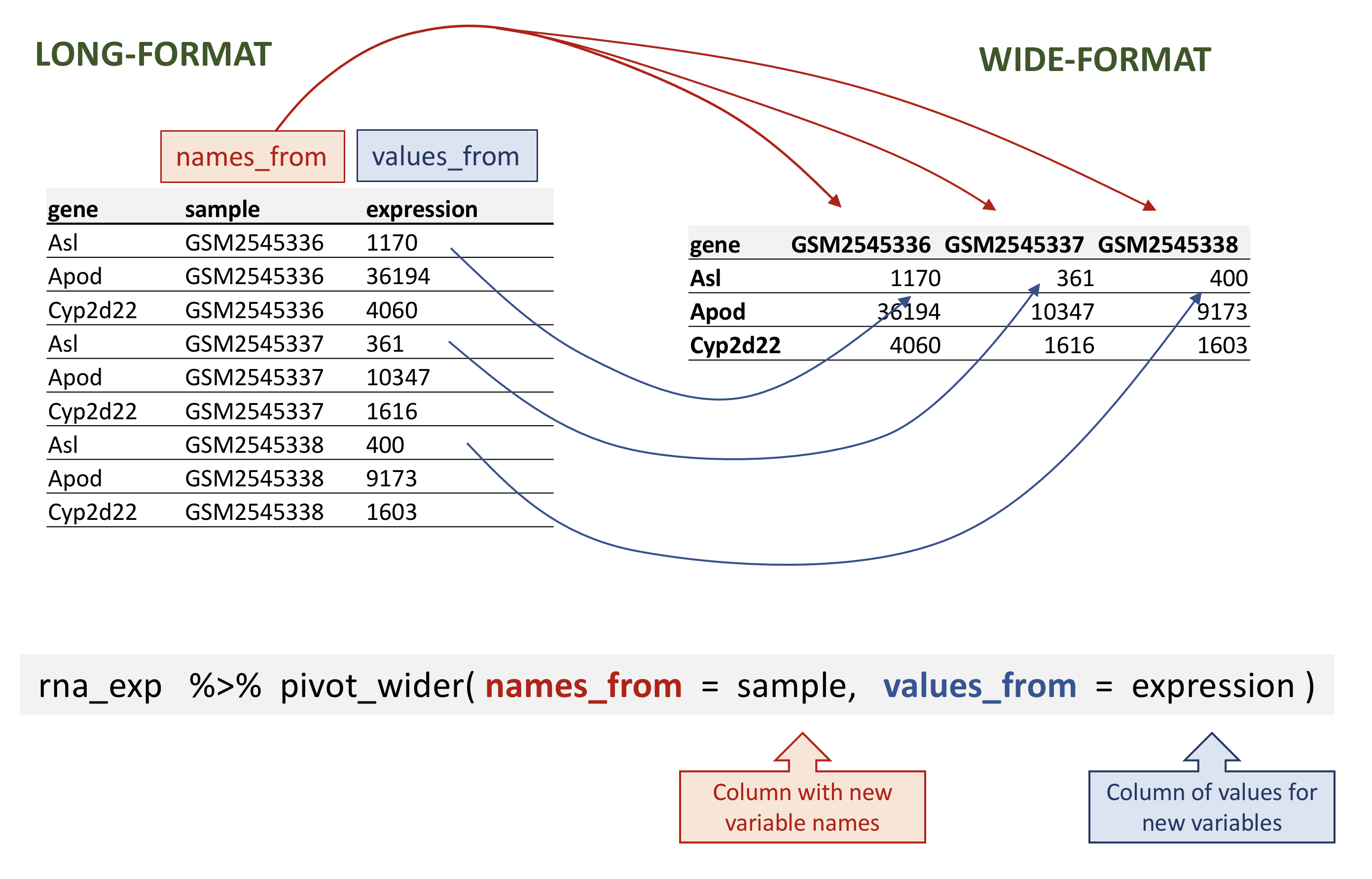
## # ℹ 32,418 more rowspivot_wider takes the following three main arguments:
- the data to be transformed;
- the
names_fromcolumn name whose values will become new column names; - the
values_fromcolumn name whose values will fill the new columns.
pivot_wider() generates a new table with 1474 gene for 22 samples -
one row for each gene, one column for each sample. We can also
directly pipe the data into the pivot_wider(), as illustrated below:
## # A tibble: 1,474 × 23
##    gene    GSM2545336 GSM2545337 GSM2545338 GSM2545339 GSM2545340 GSM2545341
##    <chr>        <dbl>      <dbl>      <dbl>      <dbl>      <dbl>      <dbl>
##  1 Asl           1170        361        400        586        626        988
##  2 Apod         36194      10347       9173      10620      13021      29594
##  3 Cyp2d22       4060       1616       1603       1901       2171       3349
##  4 Klk6           287        629        641        578        448        195
##  5 Fcrls           85        233        244        237        180         38
##  6 Slc2a4         782        231        248        265        313        786
##  7 Exd2          1619       2288       2235       2513       2366       1359
##  8 Gjc2           288        595        568        551        310        146
##  9 Plp1         43217     101241      96534      58354      53126      27173
## 10 Gnb4          1071       1791       1867       1430       1355        798
## # ℹ 1,464 more rows
## # ℹ 16 more variables: GSM2545342 <dbl>, GSM2545343 <dbl>, GSM2545344 <dbl>,
## #   GSM2545345 <dbl>, GSM2545346 <dbl>, GSM2545347 <dbl>, GSM2545348 <dbl>,
## #   GSM2545349 <dbl>, GSM2545350 <dbl>, GSM2545351 <dbl>, GSM2545352 <dbl>,
## #   GSM2545353 <dbl>, GSM2545354 <dbl>, GSM2545362 <dbl>, GSM2545363 <dbl>,
## #   GSM2545380 <dbl>
We can now easily compare the gene expression levels in different samples.
Note that the pivot_wider() function comes with an optional
values_fill argument that can be useful when dealing with missing
values. Let’s imagine that for some reason, we had some missing
expression values for some genes in certain samples. In the following
example, the gene Cyp2d22 has only one expression value, in GSM2545338
sample.
rna_with_missing_values <- rna |>
  select(gene, sample, expression) |>
  filter(gene %in% c("Asl", "Apod", "Cyp2d22")) |>
  filter(sample %in% c("GSM2545336", "GSM2545337", "GSM2545338")) |>
  arrange(sample) |>
  filter(!(gene == "Cyp2d22" & sample != "GSM2545338"))
rna_with_missing_values
## # A tibble: 7 × 3
## gene sample expression
## <chr> <chr> <dbl>
## 1 Asl GSM2545336 1170
## 2 Apod GSM2545336 36194
## 3 Asl GSM2545337 361
## 4 Apod GSM2545337 10347
## 5 Asl GSM2545338 400
## 6 Apod GSM2545338 9173
## 7 Cyp2d22 GSM2545338 1603By default, the pivot_wider() function will add NA for missing values.
## # A tibble: 3 × 4
##   gene    GSM2545336 GSM2545337 GSM2545338
##   <chr>        <dbl>      <dbl>      <dbl>
## 1 Asl           1170        361        400
## 2 Apod         36194      10347       9173
## 3 Cyp2d22         NA         NA       1603
But in some cases, we may wish to fill in the missing values by setting values_fill
to a specific value.
rna_with_missing_values |>
  pivot_wider(names_from = sample,
              values_from = expression,
              values_fill = 0)
## # A tibble: 3 × 4
## gene GSM2545336 GSM2545337 GSM2545338
## <chr> <dbl> <dbl> <dbl>
## 1 Asl 1170 361 400
## 2 Apod 36194 10347 9173
## 3 Cyp2d22 0 0 16035.8.2 Pivoting data into a longer format
The opposing situation could occur if we had been provided with data
in the form of rna_wide, where the sample IDs are column names, but
we wished to treat them as values of a sample variable instead.
In this situation we are using the column names and turn them into a
pair of new variables and need to arrange the expression values
accordingly in a new variable. This can be done with the
pivot_longer() function. It takes the following four main arguments:
- the data to be transformed;
- the new
names_tocolumn we wish to create and populate with the current column names; - the new
values_tocolumn we wish to create and populate with current values; - the names of the columns to be used to populate the
names_toandvalues_tovariables (or altarnatively, those to drop using a-).
To recreate rna_long from rna_long we would create a key
called sample and value called expression and use all columns
except gene for the key variable. Here we drop gene column
with a minus sign.
Notice how the new variable names are to be quoted here.
## # A tibble: 32,428 × 3
##    gene  sample     expression
##    <chr> <chr>           <dbl>
##  1 Asl   GSM2545336       1170
##  2 Asl   GSM2545337        361
##  3 Asl   GSM2545338        400
##  4 Asl   GSM2545339        586
##  5 Asl   GSM2545340        626
##  6 Asl   GSM2545341        988
##  7 Asl   GSM2545342        836
##  8 Asl   GSM2545343        535
##  9 Asl   GSM2545344        586
## 10 Asl   GSM2545345        597
## # ℹ 32,418 more rows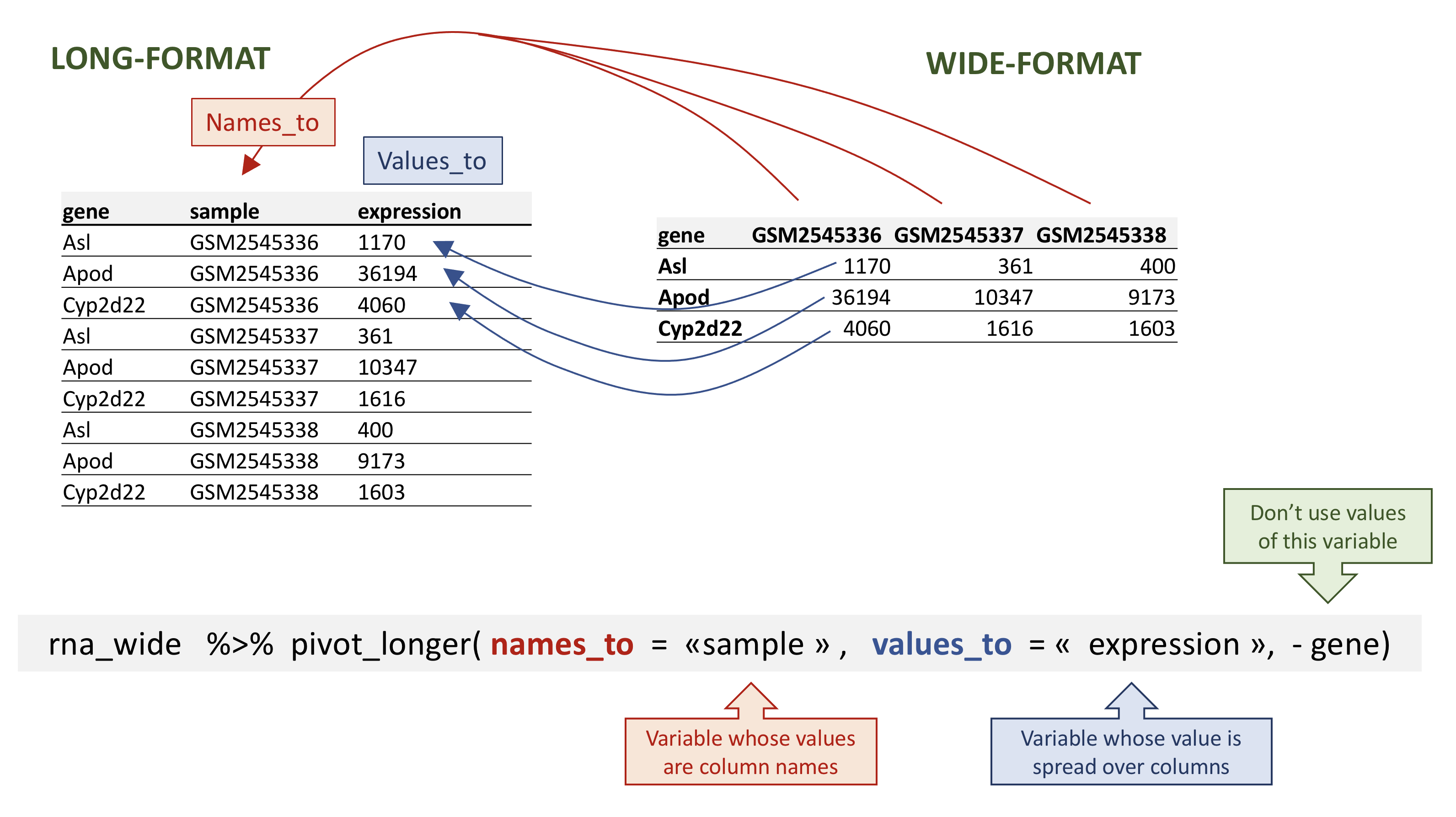
Note that if we had missing values in the wide-format, the NA would be
included in the new wide format. Pivoting to wider and longer formats can
be a useful way to balance out a dataset so every replicate has the same composition.
wide_with_NA <- rna_with_missing_values |>
  pivot_wider(names_from = sample,
              values_from = expression)
wide_with_NA
## # A tibble: 3 × 4
## gene GSM2545336 GSM2545337 GSM2545338
## <chr> <dbl> <dbl> <dbl>
## 1 Asl 1170 361 400
## 2 Apod 36194 10347 9173
## 3 Cyp2d22 NA NA 1603## # A tibble: 9 × 3
## gene sample expression
## <chr> <chr> <dbl>
## 1 Asl GSM2545336 1170
## 2 Asl GSM2545337 361
## 3 Asl GSM2545338 400
## 4 Apod GSM2545336 36194
## 5 Apod GSM2545337 10347
## 6 Apod GSM2545338 9173
## 7 Cyp2d22 GSM2545336 NA
## 8 Cyp2d22 GSM2545337 NA
## 9 Cyp2d22 GSM2545338 1603We could also have used a specification for what columns to
include. This can be useful if you have a large number of identifying
columns, and it’s easier to specify what to gather than what to leave
alone. Here the starts_with() function can help to retrieve sample
names without having to list them all!
Another possibility would be to use the : operator!
## # A tibble: 32,428 × 3
##    gene  sample     expression
##    <chr> <chr>           <dbl>
##  1 Asl   GSM2545336       1170
##  2 Asl   GSM2545337        361
##  3 Asl   GSM2545338        400
##  4 Asl   GSM2545339        586
##  5 Asl   GSM2545340        626
##  6 Asl   GSM2545341        988
##  7 Asl   GSM2545342        836
##  8 Asl   GSM2545343        535
##  9 Asl   GSM2545344        586
## 10 Asl   GSM2545345        597
## # ℹ 32,418 more rows## # A tibble: 32,428 × 3
## gene sample expression
## <chr> <chr> <dbl>
## 1 Asl GSM2545336 1170
## 2 Asl GSM2545337 361
## 3 Asl GSM2545338 400
## 4 Asl GSM2545339 586
## 5 Asl GSM2545340 626
## 6 Asl GSM2545341 988
## 7 Asl GSM2545342 836
## 8 Asl GSM2545343 535
## 9 Asl GSM2545344 586
## 10 Asl GSM2545345 597
## # ℹ 32,418 more rows► Question
Subset genes located on X and Y chromosomes from the rna data.frame
and create a new (wide) data.frame with sex as columns,
chromosome_name as rows, containing the mean expression of genes
located in each chromosome as the values, as shown below.
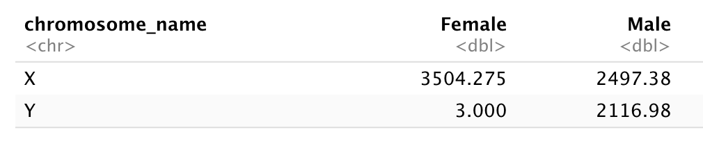
You will need to summarize before reshaping!
► Solution
► Question
Now take that data frame and transform it with pivot_longer() so
each row is a unique chromosome_name by gender combination.
► Solution
► Question
Use the rna dataset to create an new table were each row represents
the mean expression levels of genes and columns represent the
different timepoints.
► Solution
► Question
Use the previous data frame containing mean expression levels per timepoint and create a new column containing fold-changes between timepoint 8 and timepoint 0, and fold-changes between timepoint 8 and timepoint 4. Convert this table in a long-format table gathering the foldchanges calculated.
► Solution
5.9 Exporting data
Now that you have learned how to use dplyr to extract
information from or summarize your raw data, you may want to export
these new data sets to share them with your collaborators or for
archival.
Similar to the read_csv() function used for reading CSV files into
R, there is a write_csv() function that generates CSV files from
data frames.
Before using write_csv(), we are going to create a new folder,
data_output, in our working directory that will store this generated
dataset. We don’t want to write generated datasets in the same
directory as our raw data. It’s good practice to keep them
separate. The data folder should only contain the raw, unaltered
data, and should be left alone to make sure we don’t delete or modify
it. In contrast, our script will generate the contents of the
data_output directory, so even if the files it contains are deleted,
we can always re-generate them.
In preparation for our next lesson on plotting, we are going to prepare a table representing for each gene, the fold-changes (in log values) between timepoint 8 and timepoint 0, and the fold-changes between timepoint 8 and timepoint 0.
rna_fc <- rna |>
  mutate(expression_log = log(expression)) |>
  group_by(gene, time) |>
  summarize(mean_exp = mean(expression_log)) |>
  pivot_wider(names_from = time,
              values_from = mean_exp) |>
  mutate(time_8_vs_0 = `8` - `0`, time_4_vs_0 = `4` - `0`) |>
  select(gene, time_8_vs_0, time_4_vs_0)
## `summarise()` has regrouped the output.
## ℹ Summaries were computed grouped by gene and time.
## ℹ Output is grouped by gene.
## ℹ Use `summarise(.groups = "drop_last")` to silence this message.
## ℹ Use `summarise(.by = c(gene, time))` for per-operation grouping (`?dplyr::dplyr_by`) instead.## # A tibble: 1,474 × 3
## # Groups: gene [1,474]
## gene time_8_vs_0 time_4_vs_0
## <chr> <dbl> <dbl>
## 1 AI504432 -0.0248 0.0523
## 2 AW046200 -0.650 -0.0348
## 3 AW551984 0.232 -0.428
## 4 Aamp 0.0271 0.0522
## 5 Abca12 -0.116 -0.114
## 6 Abcc8 -0.114 0.0163
## 7 Abhd14a -0.309 -0.0800
## 8 Abi2 0.0110 -0.000894
## 9 Abi3bp -0.432 -0.107
## 10 Abl2 -0.0188 -0.0550
## # ℹ 1,464 more rowsWe can save the table as a CSV file in our data_output
folder.
5.10 Additional exercises
► Question
We are going to re-analyse beer consumption in 48 individuals using
dplyr. The data are available in the rWSBIM1207 package. The data
illustrated the fictive beer consumption in litres per year at
different age according to gender and employment.
- Load the
rWSBIM1207package. If the package isn’t installed of its version is older than 0.1.1, install it from theUCLouvain-CBIO/rWSBIM1207GitHub repository using theBiocManager::install()function. - Directly load the data by typing
Remove observations with missing values.
Using the
Year,MonthandDaycolumns, create a new columnDateusingdplyr::mutateandlubridate::ymd. What is the class ofDate?Create a new table, containing observations for women older than 35 years old, employed, and select all columns except Day, Month and Year, and order in descending value of consumption of beers.
Export the new table to a
csvfile.
Beer consumption analysis:
- Does employment status have an impact on beer consumption?
- Do men drink more than women?
- Does employment status have an influence on beer consumption according to gender?
- Do men drink more than women according to age and employment status?
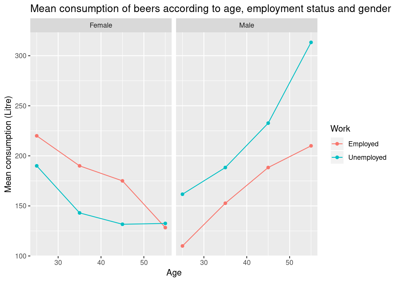
As we can see from the last exercise, it become difficult to read and interpret multiple results. In the next chapter, we will see how to complement such analysis questions with visualisations such as the following one, that clearly highlight important patterns in our data.
Figure 5.1: Visualisation of beer consumption, highlighting different patterns of beer consumption in employed and unemployed males and females.
► Question
The Cancer Genome Atlas (TCGA) is a large scale effort that has collected high throughput biology data from hundreds of patients samples. In this exercise, we are going to analyse the clinical variables recorded for a subset of the patients.
Load the
rWSBIM1207package. If the package isn’t installed of its version is older than 0.1.1, install it from theUCLouvain-CBIO/rWSBIM1207' GitHub repository using thedevtools::install_github` function.Using the
clinical1.csv()function fromrWSBIM1207, find the path theclinical1.csvfile and read it to produce adata.framenamedclinical.Familiarise yourself with the data.
Create a smaller data frame called
clinical_minicontaining only the columns corresponding topatientID,gender,age_at_diagnosis,smoking_history,number_pack_years_smoked,year_of_tobacco_smoking_onset, andstopped_smoking_year.Calculate the number of males and females in the cohort.
Create a new variable
years_at_diagnosiscorresponding to the age at diagnosis converted from days into years.Calculate the mean and median age at diagnosis (in years). Pay attention to missing values!
Calculate the mean and median age at diagnosis for males and females.
How many patient were diagnosed before 50 years?
Compare the mean age at diagnosis between current smoker and lifelong non-smoker.
Select patients who stopped smoking more than 15 years ago and calculate the number of smoking years for these cases. Display only cases for which you were able to calculate the data.
How many of them smoked less than 5 years?
Try to recreate the following table, reporting the number of smokers and lifelong-non smoker between males and females. Note: the layout can be different.
| gender | current smoker | lifelong non-smoker |
|---|---|---|
| female | 51 | 55 |
| male | 69 | 20 |
► Question
Using the interroA.csv() function from the rWSBIM1207 package to
get the path to the spreadsheet file, read the data into R using the
read_csv function. This data is in the wide format, with the results
of each test stored as a separate column.
Using the appropriate pivot function, convert the data into a long
table with a column interro informing which test that line refers to
and a column result with the student’s mark.
► Question
Make sure you have rWSBIM1207 version >= 0.1.16 and load the 2022
Belgian road accidents statistics and the associated metadata,
describing the variables. The path to the former as an rds file is
available with road_accidents_be_2022.rds(). The
road_accidents_be_meta.csv() returns the path to the metadata csv
file.
The data provides the Number of killed, seriously injured, slightly injured and uninjured victims of road accidents, by age group, type of user, sex and various characteristics of the accident in Belgium in 20222.
Using the appropriate functions, load both files into R and familiarise yourself with the data.
Compare the numbers for man and women over the hours of the day for all age classes. Ignore any unknown information.
Compare the number of victims in the different provinces. Do this comparison for the different type of victims. Ignore any unknown information.
Come up with additional question/comparisons that you could ask these data.
Page built: 2026-04-02 using R version 4.5.0 (2025-04-11)