Chapter 10 Additional programming concepts
Learning Objectives
Learn programming concepts, including
- how to handle conditions
- iteration of data structures
- good coding practice
- code re-use through functions
When the size and the complexity of the data increases, or the data science question of interest becomes more complex, the data analysis techniques as we have seen them so far need to be complemented with programming techniques. From a data science point of view, there is no clear delimitation between data analysis and (data) programming, both morphing into each other19 A fundamental difference however is how data analysis and programming are taught. When it comes to researchers, and biomedical researchers in particular, teaching programming to analyse data isn’t successful. Teaching data analysis to eventually programme with data, however, has proven a successful strategy..
This chapter will introduce some additional programming skills and demonstrate how to use them in the context of high troughput omics data.
10.1 Writing clean code
Writing clean code means writing easily readable code, hence easily understandable code and, eventually code with less bugs. One easy way to achieve this is through consistency, i.e. stick to a style guide. The issue is that there are several style guides available, often with conflicting suggestions. Two widely used ones are the Bioconductor style guide and Hadley Wickhams’s R Style Guide. The advice from for naming variables seen in the first and second chapters are also relevant.
Here are a couple of suggestions:
- Use
<-to assign variables. Use=is also valid, but make sure that you stick with one. - Use either camel case (
camelCaseNaming) of snake case (snake_case_naming), and avoid using dots (don’t usedot.variable.names). These conventions apply to functions, variables and files (for the latter, a-instead of_is also acceptable). - Always spell out
TRUEandFALSE, and resist the temptation to useTandFinstead20TRUEandFALSEare reserved words; one can’t use them as variable names. This however doesn’t hold forTandF. One can useTandFas regular variable names such, as for example,T <- FALSEandF <- TRUE!. - Use 4 spaces for indenting. No tabs.
- No lines longer than 80 characters.
- Use spaces around binary operators.
- No spaces between a function name and the opening parenthesis.
Another good advise is to avoid re-writing the same code many times. We will see below two strategies to do that, namely iteration and writing new functions. This firstly reduces the amount of code typed and hence the number of bugs, but more importantly enables consistency. If something in your code changes, there’s only one change and it applies everywhere, rather than doing that same change repeatedly (at the first of adding bugs and to miss some updates).
When writing code, keep it simple and short21 The official motto is KISS, keep your functions simple, stupid, widely used in programming.. Ideally, the code should be evident. But when the questions tackled are not trivial, is becomes essential to add comments to clarify aspects of the script/program. Make sure to use them to describe why something is done, rather than explaining how things are done (which is tyically best done by the code itself).
A general guideline to avoid bugs is to apply defensive programming:
- making the code work in a predicable manner
- writing code that fails in a well-defined manner
- if something weird happens, either properly deal with it, or it fail quickly and loudly
Here are some examples of how to do this:
use functions like
is.numeric(x),is.character(x),is.data.frame(x), … but make sure that the variable you are going to use is of the expected type.Make sure the length or dimensions of what you are going to use are what you expect:
- Failing fast and well! Wrap such test in
stopifnot(), so that if they fail, you get immediately an error, rather than risking that you code fails later with obscure error messages or, worse, the code runs to completion but returns meaningless results.
10.2 Iteration
Iteration describes the situtation when a specific operation has to be
repeated many times on different inputs of the same type. For example,
if we have a vector of numeric x shown below,
## [1] 1 2 3 4 5 6 7 8 9 10and we wanted to apply the logarithm operation on each element of x,
it wouldn’t be convenient to type
log(1)
log(2)
log(3)
...
log(10)
The concept of iteration allows us to program the following command:
Repeat
logfor each value of my inputx.
or more formally
Repeat
log(i)whereitakes in turn each value of my inputx.
We will see different ways of implementing such an iteration.
Using a for loop
## [1] 0
## [1] 0.6931472
## [1] 1.098612
## [1] 1.386294
## [1] 1.609438
## [1] 1.791759
## [1] 1.94591
## [1] 2.079442
## [1] 2.197225
## [1] 2.302585
The loop above only prints the results on screen. They aren’t stored
and are lost for any further re-use, which would be very annoying if
it took much more time to perform all the calculations. In the code
chunk below, we are going to first inititalise a vector with the
appropriate number of NA values and, at each iteration, we then
store the result. We however now need to change our loop and iterate
of the indices of the input vector, so that we can re-use these
indices to save the results in the output vector.
##  [1] 0.0000000 0.6931472 1.0986123 1.3862944 1.6094379 1.7917595 1.9459101
##  [8] 2.0794415 2.1972246 2.3025851
Using the apply function
The apply family of functions implements our defintion of iteration quite literally
Repeat
logfor each value of my inputx
is reformulated as
For each value of my input
x, applylog
and coded as
##  [1] 0.0000000 0.6931472 1.0986123 1.3862944 1.6094379 1.7917595 1.9459101
##  [8] 2.0794415 2.1972246 2.3025851
There are three such function that apply a function iteratively:
sapplyiterates over a vector and returns a new vector of the same length as the input vector22 This is a simplification of howsapplyworks, that is partly defined by the thesimplifyargument and whether the result of applying the function on each element of the input can be returned as a vector. The alternative is to return alist, likelapply..lapplyiterates over a linear input (a vector of a list) and returns a list of the same length as the input.applyiterates of the rows or the columns of adata.frameormatrixand returns a list or vector or approritate length (number of rows or columns). The dimension over which the iterations proceeds is defined by the second argument, where1defines rows and2defined columns23 This generalises to arrays with more than 2 dimensions..
When performing the same operations in different ways (using different
implementations), it is essential to verify that the results are
identical or, if not, at least compatible. The most direct way to do
the former is to use the identical function:
## [1] TRUEThe purrr package a set of map functions similar to the apply
set described above.
Vectorisation
We must not forget the obvious, which is vectorisation. Many R functions work by default iteratively on every element of a vectors, i.e. they work irrespectively whether the vector is of length 124 A vector of length 1 would be called a scalar in other programming languages. or longer.
##  [1] 0.0000000 0.6931472 1.0986123 1.3862944 1.6094379 1.7917595 1.9459101
##  [8] 2.0794415 2.1972246 2.3025851
And, as before, we check that we obtain identical results:
## [1] TRUEWhich iteration to use?
Even though they produce the same result, the iteration strategies above aren’t equal, and some should be preferred in different situations.
When a vectorised solution exists, this is the one that should be chosen. It is by far the fastest solution, but only applicable to existing vectorised functions. If you were to write your own function to iterate over, it is advisable to write a vectorised function.
The apply functions are extremely convenient and concise, and hence widely used. They have a couple of advantages, including that there is no need to explicitly initialise a result variable and that they can easily be parallelised.
For loops are the most generic solution for iteration, and they require to initialise the result variable that will be populated during the loop. As opposed to popular belief, they aren’t slower than using apply functions. They are however the best solution if, during the iteration, one has the access another element than the one currently processed (typically, if
iis the counter, accessingi + 1ori - 1).
► Question
Use the expressions.csv() function from the rWSBIM1207 package to
get the path to 5 csv files containing gene expression data
for a single gene and hundreds of patience. Read all data in and
combine them into a single dataframe.
Before starting, open at least two of these files to familiarise yourself with their structure and identify how and with what function they need to be combined.
► Solution
10.3 Conditionals
When an operation has to be executed when a condition is met, one
typically uses a if and else construct:
if (CONDITION) {
   ## DO SOMETHING
} else {
  ## DO SOMETHING ELSE
}
For examples
## [1] -0.6264538## [1] -0.4676802But note that in the example above, it would be much better to
simplify the code and use the absolute value of x before taking the
log, which will generalise the calculation for positive and negative
values …
## [1] -0.4676802… and works for vectors of any length thanks to vectorisation.
##  [1] -1.6947599 -0.1795710  0.4670498 -1.1101553 -0.1978799 -0.7186105
##  [7] -0.3033716 -0.5520273 -1.1861709  0.4132885
There are also in-line, vectorised versions of the if/else
statements seen above: the ifelse function that ships with the
base package, and if_else from dplyr. Both work similarly (the
differences are beyond the scope of this course) and have the form:
if_else(condition, true, false)- where
conditionis the condition to be tested, and will return eitherTRUEorFALSE; -
trueis the expression that is executed if the condition isTRUE; -
falseis the expression that is executed otherwise (i.e if the condition isFALSE).
Here is an example, that will return 1 if x is strictly positive,
and 0 otherwise:
## [1] 1The function being vectorised, the condition can be a vector of length greater than 1:
##  [1]  0.38984324 -0.62124058 -2.21469989  1.12493092 -0.04493361 -0.01619026
## [7] 0.94383621 0.82122120 0.59390132 0.91897737## [1] 1 0 0 1 0 0 1 1 1 1The vectorised conditional functions can directly be used in a standard data analysis pipeline:
## # A tibble: 5 × 2
##   x          y
##   <chr>  <dbl>
## 1 a     -0.626
## 2 b      0.184
## 3 c     -0.836
## 4 d      1.60
## 5 e 0.330## # A tibble: 5 × 3
## x y z
## <chr> <dbl> <dbl>
## 1 a -0.626 0
## 2 b 0.184 1
## 3 c -0.836 0
## 4 d 1.60 1
## 5 e 0.330 110.4 Writing new functions
A function is composed of a name, inputs (inside the parenthesis), a
body (between curly brackets) and an ouput (last statement or variably
inside the return statement).
my_fun <- function(x, y) {
    message("First input: ", x)
    message("Second input: ", y)
    z <- x * abs(y)
    return(z)
}
my_fun(2, -5)
## First input: 2## Second input: -5## [1] 10► Question
Complete the following function. It is supposed to take two inputs,
x and y and, depending whether the x > y or x <= y, it generates
the permutation sample(x, y) in the first case or draws a sample
from rnorm(1000, x, y) in the second case. Finally, it returns the
sum of all values.
fun <- function(x, y) {
    res <- NA
    if (   ) {
        res <- sample(, )
    } else {
        res <- rnorm(, , )
    }
    return()
}
To check your answer, run it with inputs 5, 15 and 15, 5, after
setting the random number generator to 1 each time with set.seed(1)
and you should get 4825.2778709 and 23.
► Solution
10.5 Pattern matching
One skill that comes handy more often than not is the ability to find
patterns in text and replace these. We are going to see two functions
out of many to perform such tasks. As an illustration, we are going to
mine a vector or peptides identified by mass spectrometry. The data
can be loaded from the rWSBIM1207 data:
## [1] 26796## [1] "aAAGEAk" "VTEEAk" "aSGDPGk" "sAAAEAk" "aANAEGk" "aAAEEAR"- Among the 26796 petides, which ones contain the pattern
"AAGE"?
## [1] 1 7026 17140 21912 23423 24947 25257 26658## [1] "aAAGEAk" "aFHGAAGEAGAAFGNHGANR" "eAIDAAGEGGR"
## [4] "sAAGEFADDPcSSVkR" "eAAGEGPVLYEDPPDQk" "eIEAAGEk"
## [7] "dVQELYAAGENR" "sAAGEFADDPcSSVk"## [1] TRUE FALSE FALSE FALSE FALSE FALSE- Replace a pattern by another string.
## [1] "aAAGEAk" "VTEEAk" "aSGDPGk" "sAAAEAk" "aANAEGk" "aAAEEAR"## [1] "aAAGEAk" "VTEEAk" "aSGDPGk" "sAAXXAk" "aANXXGk" "aAXXEAR"But careful that sub only replaced the first occurrence in a string!
## [1] "aAAGEAk" "VTEEAk" "aSGDPGk" "sAAAEAk" "aANAEGk" "aAAEEAR"## [1] "aXAGEAk" "VTEEXk" "aSGDPGk" "sXAAEAk" "aXNAEGk" "aXAEEAR"## [1] "aXXGEXk" "VTEEXk" "aSGDPGk" "sXXXEXk" "aXNXEGk" "aXXEEXR"10.6 Analysing data from multiple files
This exercise recapitulates the most important material that we have
seen in this course. We are going to analyse the student tests A and B
results using functionality from the dplyr package (seen in chapter
5). The student test files are available in the
rWSBIM1207 package (the interroA.csv and interroB.csv functions
return their respective paths). We want to compare how the male and
female students in groups A and B have performed. To do this, we want
to calculate the mean scores and visualise the score distributions in
each groups.
► Question
Before writing any code to answer the questions above, take a couple of minutes to think about what packages are needed to answer the questions above and identify the individual steps needed to first prepare the data needed to find the answers and then to produce the answers.
- Start by loading the
rWSBIM1207andtidyversepackage, to get all the functionality we will need.
► Solution
- Using the
interroA.csv()andinterroB.csv()functions from therWSBIM1207package, create a vector containing the two csv file names.
► Solution
- Iterate over the files and read each into an element of a list. Then, bind the two elements of the list into a single dataframe containing all results.
► Solution
- What are the mean scores for male and female students in each test
(
interro1tointerro4).
► Solution
- What are the mean scores for male and female students in each test
(
interro1tointerro4) and in each group (A and B).
► Solution
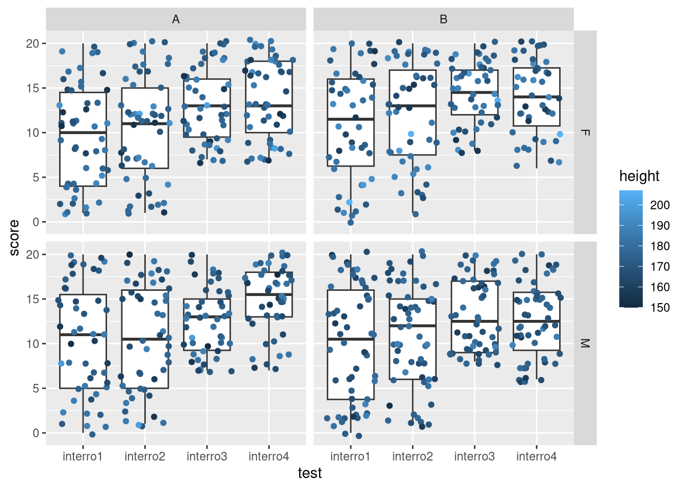
- Instead of comparing the means for the four tests in each group and gender, visualise their distributions using boxplots. In addition to the boxplots, overlay the actual score values (using the jitter geom) and colour the points based on the students height.
► Solution
10.7 Additional exercises
► Question
► Question
Write functions that convert temperatures:
- from Fahrenheit to Kelvin, where \(T_K = (T_F - 32) \times 5/9 + 273.15\)
- fom Celsius to Kelvin, where \(T_K = T_C + 273.15\)
- from Kelvin to Celsis
- from Fahrenheit to Celsius
Page built: 2026-04-02 using R version 4.5.0 (2025-04-11)