Chapter 7 Joining tables

7.1 Combining tables

Copy link

We are going to illustrate join using a common example from the bioinformatics world, where annotations about genes are scattered in different tables that have one or more shared columns. The data we are going to use are available in the course package and can be loaded as shown below.

library("rWSBIM1207")
data(jdf)

The example data is composed of pairs of tables (we have tibbles here, but this would equally work with dataframes). The first member of the pair contains protein UniProt¹¹ unique accession number (uniprot variable), the most likely sub-cellular localisation of these respective proteins (organelle variable) as well as the proteins identifier (entry).

jdf1

## # A tibble: 25 × 3
##    uniprot  organelle                             entry      
##    <chr>    <chr>                                 <chr>      
##  1 P26039   Actin cytoskeleton                    TLN1_MOUSE 
##  2 Q99PL5   Endoplasmic reticulum/Golgi apparatus RRBP1_MOUSE
##  3 Q6PB66   Mitochondrion                         LPPRC_MOUSE
##  4 P11276   Extracellular matrix                  FINC_MOUSE 
##  5 Q6PR54   Nucleus - Chromatin                   RIF1_MOUSE 
##  6 Q05793   Extracellular matrix                  PGBM_MOUSE 
##  7 P19096   Cytosol                               FAS_MOUSE  
##  8 Q9JKF1   Plasma membrane                       IQGA1_MOUSE
##  9 Q9QZQ1-2 Plasma membrane                       AFAD_MOUSE 
## 10 Q6NS46   Nucleus - Non-chromatin               RRP5_MOUSE 
## # ℹ 15 more rows

The second table contains the name of the gene that codes for the protein (gene_name variable), a description of the gene (description variable), the uniprot accession number (this is the common variable that can be used to join tables) and the species the protein information comes from (organism variable).

jdf2

## # A tibble: 25 × 4
##    gene_name description                                      uniprot organism
##    <chr>     <chr>                                            <chr>   <chr>   
##  1 Iqgap1    Ras GTPase-activating-like protein IQGAP1        Q9JKF1  Mmus    
##  2 Hspa5     78 kDa glucose-regulated protein                 P20029  Mmus    
##  3 Pdcd11    Protein RRP5 homolog                             Q6NS46  Mmus    
##  4 Tfrc      Transferrin receptor protein 1                   Q62351  Mmus    
##  5 Hspd1     60 kDa heat shock protein, mitochondrial         P63038  Mmus    
##  6 Tln1      Talin-1                                          P26039  Mmus    
##  7 Smc1a     Structural maintenance of chromosomes protein 1A Q9CU62  Mmus    
##  8 Lamc1     Laminin subunit gamma-1                          P02468  Mmus    
##  9 Hsp90b1   Endoplasmin                                      P08113  Mmus    
## 10 Mia3      Melanoma inhibitory activity protein 3           Q8BI84  Mmus    
## # ℹ 15 more rows

We now want to join these two tables into a single one containing all variables. We are going to use dplyr’s full_join function to do so, that finds the common variable (in this case uniprot) to match observations from the first and second table.

library("dplyr")
full_join(jdf1, jdf2)

## Joining with `by = join_by(uniprot)`

## # A tibble: 25 × 6
##    uniprot  organelle                       entry gene_name description organism
##    <chr>    <chr>                           <chr> <chr>     <chr>       <chr>   
##  1 P26039   Actin cytoskeleton              TLN1… Tln1      Talin-1     Mmus    
##  2 Q99PL5   Endoplasmic reticulum/Golgi ap… RRBP… Rrbp1     Ribosome-b… Mmus    
##  3 Q6PB66   Mitochondrion                   LPPR… Lrpprc    Leucine-ri… Mmus    
##  4 P11276   Extracellular matrix            FINC… Fn1       Fibronectin Mmus    
##  5 Q6PR54   Nucleus - Chromatin             RIF1… Rif1      Telomere-a… Mmus    
##  6 Q05793   Extracellular matrix            PGBM… Hspg2     Basement m… Mmus    
##  7 P19096   Cytosol                         FAS_… Fasn      Fatty acid… Mmus    
##  8 Q9JKF1   Plasma membrane                 IQGA… Iqgap1    Ras GTPase… Mmus    
##  9 Q9QZQ1-2 Plasma membrane                 AFAD… Mllt4     Isoform 1 … Mmus    
## 10 Q6NS46   Nucleus - Non-chromatin         RRP5… Pdcd11    Protein RR… Mmus    
## # ℹ 15 more rows

In the examples above, each observation of the jdf1 and jdf2 tables are uniquely identified by their UniProt accession number. Such variables are called keys. Keys are used to match observations across different tables.

In case none of the variable names match, those to be used can be set manually using the by argument, as shown below with the jdf1 (as above) and jdf3 tables, where the UniProt accession number is encoded using a different capitalisation.

names(jdf3)

## [1] "gene_name"   "description" "UniProt"     "organism"

full_join(jdf1, jdf3, by = c("uniprot" = "UniProt"))

## # A tibble: 25 × 6
##    uniprot  organelle                       entry gene_name description organism
##    <chr>    <chr>                           <chr> <chr>     <chr>       <chr>   
##  1 P26039   Actin cytoskeleton              TLN1… Tln1      Talin-1     Mmus    
##  2 Q99PL5   Endoplasmic reticulum/Golgi ap… RRBP… Rrbp1     Ribosome-b… Mmus    
##  3 Q6PB66   Mitochondrion                   LPPR… Lrpprc    Leucine-ri… Mmus    
##  4 P11276   Extracellular matrix            FINC… Fn1       Fibronectin Mmus    
##  5 Q6PR54   Nucleus - Chromatin             RIF1… Rif1      Telomere-a… Mmus    
##  6 Q05793   Extracellular matrix            PGBM… Hspg2     Basement m… Mmus    
##  7 P19096   Cytosol                         FAS_… Fasn      Fatty acid… Mmus    
##  8 Q9JKF1   Plasma membrane                 IQGA… Iqgap1    Ras GTPase… Mmus    
##  9 Q9QZQ1-2 Plasma membrane                 AFAD… Mllt4     Isoform 1 … Mmus    
## 10 Q6NS46   Nucleus - Non-chromatin         RRP5… Pdcd11    Protein RR… Mmus    
## # ℹ 15 more rows

As can be seen above, the variable name of the first table is retained in the joined one.

full_join(jdf4, jdf5)

## Joining with `by = join_by(uniprot)`

## # A tibble: 14 × 6
##    uniprot  organelle                       entry gene_name description organism
##    <chr>    <chr>                           <chr> <chr>     <chr>       <chr>   
##  1 P26039   Actin cytoskeleton              TLN1… <NA>      <NA>        <NA>    
##  2 Q99PL5   Endoplasmic reticulum/Golgi ap… RRBP… <NA>      <NA>        <NA>    
##  3 Q6PB66   Mitochondrion                   LPPR… <NA>      <NA>        <NA>    
##  4 P11276   Extracellular matrix            FINC… <NA>      <NA>        <NA>    
##  5 Q6PR54   Nucleus - Chromatin             RIF1… <NA>      <NA>        <NA>    
##  6 Q05793   Extracellular matrix            PGBM… <NA>      <NA>        <NA>    
##  7 P19096   Cytosol                         FAS_… Fasn      Fatty acid… Mmus    
##  8 Q9JKF1   Plasma membrane                 IQGA… <NA>      <NA>        <NA>    
##  9 Q9QZQ1-2 Plasma membrane                 AFAD… <NA>      <NA>        <NA>    
## 10 Q6NS46   Nucleus - Non-chromatin         RRP5… <NA>      <NA>        <NA>    
## 11 P02468   <NA>                            <NA>  Lamc1     Laminin su… Mmus    
## 12 P08113   <NA>                            <NA>  Hsp90b1   Endoplasmin Mmus    
## 13 Q8BI84   <NA>                            <NA>  Mia3      Melanoma i… Mmus    
## 14 Q6P5D8   <NA>                            <NA>  Smchd1    Structural… Mmus

7.2 Different types of joins

Copy link

Above, we have used the full_join function, that fully joins two tables and keeps all observations, adding missing values if necessary. Sometimes, we want to be selective, and keep observations that are present in only one or both tables.

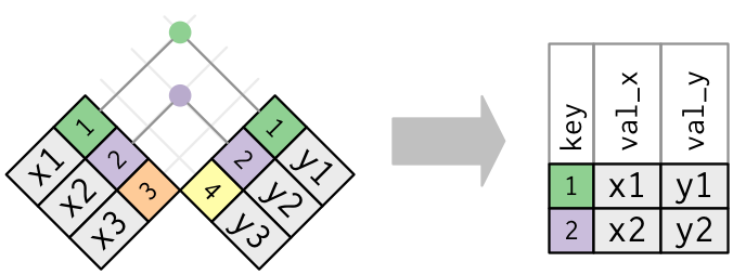
• An inner join keeps observations that are present in both tables.

Figure 7.1: An inner join matches pairs of observation matching in both tables, this dropping those that are unique to one table. Figure taken from R for Data Science.

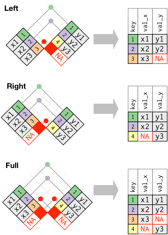
• A left join keeps observations that are present in the left (first) table, dropping those that are only present in the other.
• A right join keeps observations that are present in the right (second) table, dropping those that are only present in the other.
• A full join keeps all observations.

Figure 7.2: Outer joins match observations that appear in at least on table, filling up missing values with NA values. Figure taken from R for Data Science.

left_join(jdf4, jdf5)

## Joining with `by = join_by(uniprot)`

## # A tibble: 10 × 6
##    uniprot  organelle                       entry gene_name description organism
##    <chr>    <chr>                           <chr> <chr>     <chr>       <chr>   
##  1 P26039   Actin cytoskeleton              TLN1… <NA>      <NA>        <NA>    
##  2 Q99PL5   Endoplasmic reticulum/Golgi ap… RRBP… <NA>      <NA>        <NA>    
##  3 Q6PB66   Mitochondrion                   LPPR… <NA>      <NA>        <NA>    
##  4 P11276   Extracellular matrix            FINC… <NA>      <NA>        <NA>    
##  5 Q6PR54   Nucleus - Chromatin             RIF1… <NA>      <NA>        <NA>    
##  6 Q05793   Extracellular matrix            PGBM… <NA>      <NA>        <NA>    
##  7 P19096   Cytosol                         FAS_… Fasn      Fatty acid… Mmus    
##  8 Q9JKF1   Plasma membrane                 IQGA… <NA>      <NA>        <NA>    
##  9 Q9QZQ1-2 Plasma membrane                 AFAD… <NA>      <NA>        <NA>    
## 10 Q6NS46   Nucleus - Non-chromatin         RRP5… <NA>      <NA>        <NA>

right_join(jdf4, jdf5)

## Joining with `by = join_by(uniprot)`

## # A tibble: 5 × 6
##   uniprot organelle entry     gene_name description                     organism
##   <chr>   <chr>     <chr>     <chr>     <chr>                           <chr>   
## 1 P19096  Cytosol   FAS_MOUSE Fasn      Fatty acid synthase             Mmus    
## 2 P02468  <NA>      <NA>      Lamc1     Laminin subunit gamma-1         Mmus    
## 3 P08113  <NA>      <NA>      Hsp90b1   Endoplasmin                     Mmus    
## 4 Q8BI84  <NA>      <NA>      Mia3      Melanoma inhibitory activity p… Mmus    
## 5 Q6P5D8  <NA>      <NA>      Smchd1    Structural maintenance of chro… Mmus

inner_join(jdf4, jdf5)

## Joining with `by = join_by(uniprot)`

## # A tibble: 1 × 6
##   uniprot organelle entry     gene_name description         organism
##   <chr>   <chr>     <chr>     <chr>     <chr>               <chr>   
## 1 P19096  Cytosol   FAS_MOUSE Fasn      Fatty acid synthase Mmus

7.3 Multiple matches

Copy link

Sometimes, keys aren’t unique. In the jdf6 table below, we see that the accession number Q99PL5 is repeated twice. According to this table, the ribosomial protein binding protein 1 localises in the endoplasmic reticulum (often abbreviated ER) and in the Golgi apparatus (often abbreviated GA).

jdf6

## # A tibble: 5 × 4
##   uniprot organelle             entry       isoform
##   <chr>   <chr>                 <chr>         <dbl>
## 1 P26039  Actin cytoskeleton    TLN1_MOUSE        1
## 2 Q99PL5  Endoplasmic reticulum RRBP1_MOUSE       1
## 3 Q99PL5  Golgi apparatus       RRBP1_MOUSE       2
## 4 Q6PB66  Mitochondrion         LPPRC_MOUSE       1
## 5 P11276  Extracellular matrix  FINC_MOUSE        1

If we now want to join jdf6 and jdf2, the variables of the latter will be duplicated.

inner_join(jdf6, jdf2)

## Joining with `by = join_by(uniprot)`

## # A tibble: 5 × 7
##   uniprot organelle             entry     isoform gene_name description organism
##   <chr>   <chr>                 <chr>       <dbl> <chr>     <chr>       <chr>   
## 1 P26039  Actin cytoskeleton    TLN1_MOU…       1 Tln1      Talin-1     Mmus    
## 2 Q99PL5  Endoplasmic reticulum RRBP1_MO…       1 Rrbp1     Ribosome-b… Mmus    
## 3 Q99PL5  Golgi apparatus       RRBP1_MO…       2 Rrbp1     Ribosome-b… Mmus    
## 4 Q6PB66  Mitochondrion         LPPRC_MO…       1 Lrpprc    Leucine-ri… Mmus    
## 5 P11276  Extracellular matrix  FINC_MOU…       1 Fn1       Fibronectin Mmus

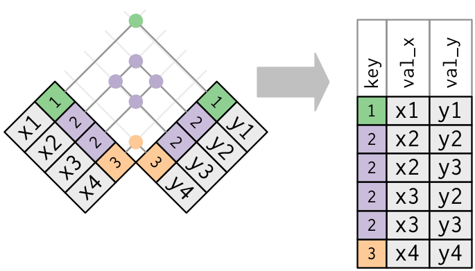
In the case above, repeating is useful, as it completes jdf6 with correct information from jdf2. One needs however to be careful when duplicated keys exist in both tables. Below, we create an inner join between jdf6 and jdf7, both having duplicated Q99PL5 entries.

inner_join(jdf6, jdf7)

## Joining with `by = join_by(uniprot)`

## Warning in inner_join(jdf6, jdf7): Detected an unexpected many-to-many relationship between `x` and `y`.
## ℹ Row 2 of `x` matches multiple rows in `y`.
## ℹ Row 1 of `y` matches multiple rows in `x`.
## ℹ If a many-to-many relationship is expected, set `relationship = "many-to-many"` to silence
##   this warning.

## # A tibble: 4 × 9
##   uniprot organelle     entry isoform gene_name description organism isoform_num
##   <chr>   <chr>         <chr>   <dbl> <chr>     <chr>       <chr>          <dbl>
## 1 Q99PL5  Endoplasmic … RRBP…       1 Rrbp1     Ribosome-b… Mmus               1
## 2 Q99PL5  Endoplasmic … RRBP…       1 Rrbp1     Ribosome-b… Mmus               2
## 3 Q99PL5  Golgi appara… RRBP…       2 Rrbp1     Ribosome-b… Mmus               1
## 4 Q99PL5  Golgi appara… RRBP…       2 Rrbp1     Ribosome-b… Mmus               2
## # ℹ 1 more variable: measure <dbl>

► Solution

jdf6 has two entries, one for each possible sub-cellular localisation of the protein. jdf7 has also two entries, referring to two different quantitative measurements (variable measure). When joining the duplicated keys, you get all possible combinations.

Figure 7.3: Joins with duplicated keys in both tables, producing all possible combinations. Figure taken from R for Data Science.

In this case, we obtain wrong information: both proteins in the ER and in the GA both have value 102 and 3.

7.4 Matching across multiple keys

Copy link

So far, we have matched tables using a single key (possibly with different names in the two tables). Sometimes, it is necessary to match tables using multiple keys. A typical example is when multiple variables are needed to discriminate different rows in a tables.

Following up from the last example, we see that the duplicated UniProt accession numbers in the jdf6 and jdf7 tables refer to different isoforms of the same RRBP1 gene. To uniquely identify isoforms, we need to consider two keys, namely the UniProt accession number (named uniprot in both tables) as well as the isoform number, called isoform and isoform_num respectively.

Because the isoform status was encoded using different variable names (which is, of course a source of confusion), jdf6 and jdf7 are only automatically joined based on the shared uniprot key. Here, we need to join using both keys and need to explicitly name the variables used for the join.

inner_join(jdf6, jdf7, by = c("uniprot" = "uniprot", "isoform" = "isoform_num"))

## # A tibble: 2 × 8
##   uniprot organelle         entry isoform gene_name description organism measure
##   <chr>   <chr>             <chr>   <dbl> <chr>     <chr>       <chr>      <dbl>
## 1 Q99PL5  Endoplasmic reti… RRBP…       1 Rrbp1     Ribosome-b… Mmus         102
## 2 Q99PL5  Golgi apparatus   RRBP…       2 Rrbp1     Ribosome-b… Mmus           3

We now see that isoform 1 localised to the ER and has a measured value of 102, while isoform 2, that localised to the GA, has a measured value of 3.

i <- grep("isoform", names(jdf7))
names(jdf7)[i] <- "isoform"
inner_join(jdf6, jdf7)

## Joining with `by = join_by(uniprot, isoform)`

## # A tibble: 2 × 8
##   uniprot organelle         entry isoform gene_name description organism measure
##   <chr>   <chr>             <chr>   <dbl> <chr>     <chr>       <chr>      <dbl>
## 1 Q99PL5  Endoplasmic reti… RRBP…       1 Rrbp1     Ribosome-b… Mmus         102
## 2 Q99PL5  Golgi apparatus   RRBP…       2 Rrbp1     Ribosome-b… Mmus           3

7.5 Merge in base R

Copy link

Above, we have used several join functions from the dplyr package as they are convenient and easy to remember. The equivalent function in the base package, that is installed with R, is the merge function. The table below shows how these are related:

Even if you decide to stick with one of these alternatives, it is important to be aware of the other one, especially given the widespread usage of merge in many packages and in R itself.

7.6 Row and column binding

Copy link

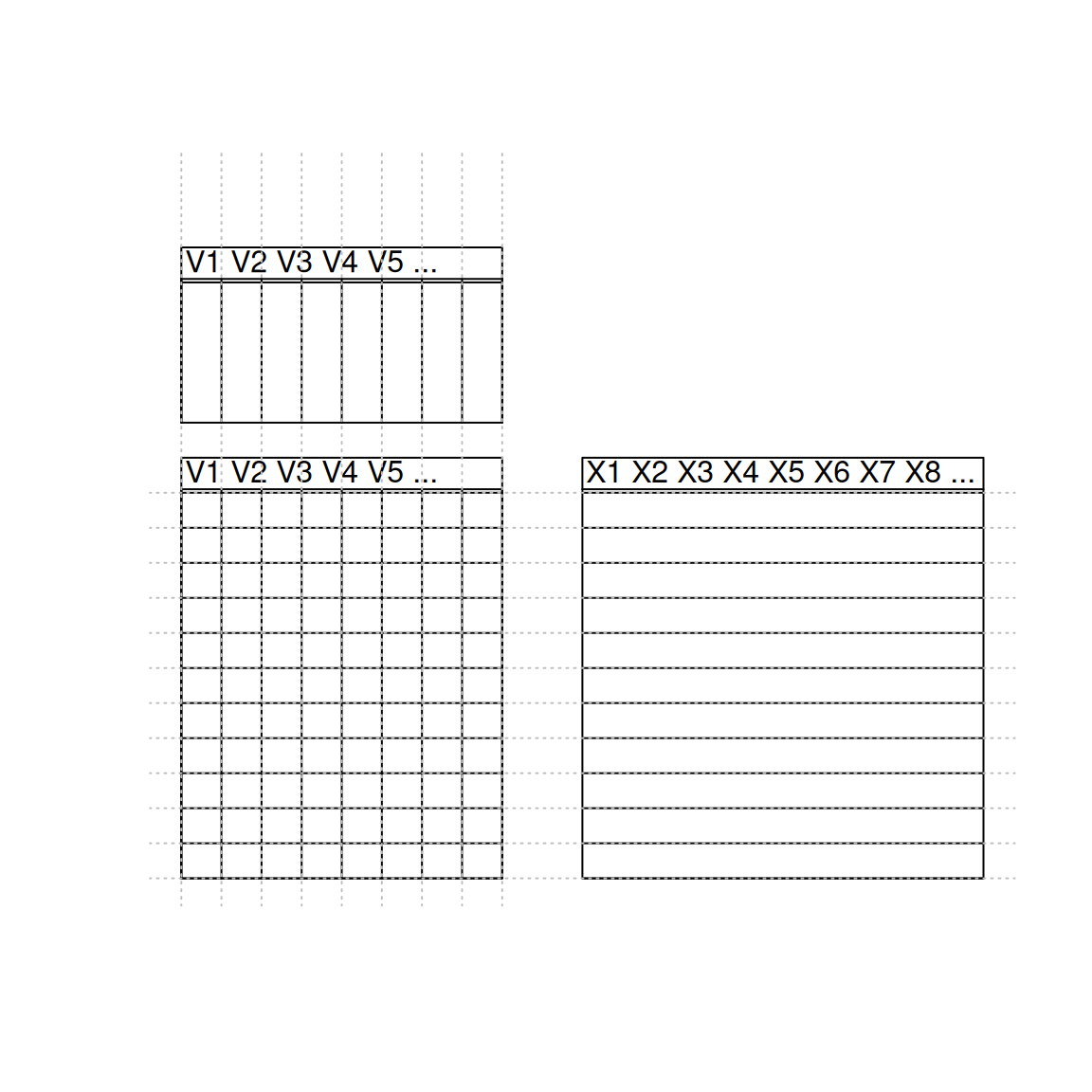
There are other two important functions in R, that can be used to combine two dataframes, but assume that these already match beforehand, as summerised in figure 7.4 below.

Figure 7.4: Matching dimension and names when binding by rows and columns.

We are going to illustrate binding by columns with dataframes d1 and d2, and then binding by rows using d2 and d3. Lets start with d1 and d2 shown below; both have the same number of columns but, and this is crucial, do not have the same column names:

d1

##   x y
## 1 1 1
## 2 2 2
## 3 3 3

d2

##   a b
## 1 4 4
## 2 5 5

While the number of columns match, the names don’t, which results in an error¹² when we use rbind:

try(rbind(d1, d2))

## Error in match.names(clabs, names(xi)) : 
##   names do not match previous names

Before rbinding two dataframes, we must assure that their number of columns and rownames match exactly:

names(d2) <- names(d1)
rbind(d1, d2)

##   x y
## 1 1 1
## 2 2 2
## 3 3 3
## 4 4 4
## 5 5 5

If we want to bind to dataframes along their columns, we must make sure that their number of rows match; rownames not hinder here:

d3

##   v1 v2 v3
## 1  1  3  5
## 2  2  4  6

cbind(d2, d3)

##   x y v1 v2 v3
## 1 4 4  1  3  5
## 2 5 5  2  4  6

Note that beyond the dimensions and column names that are required to match, the real meaning of rbind is to bind dataframes that contain observations for the same set of variables - there is more than only the column names. Below, we rbind dataframes with identical column names but different variables, which end up all being coerced into characters.

d1

##   x y
## 1 1 1
## 2 2 2
## 3 3 3

d4 <- data.frame(x = letters[1:2], y = letters[1:2])
str(rbind(d1, d4))

## 'data.frame':    5 obs. of  2 variables:
##  $ x: chr  "1" "2" "3" "a" ...
##  $ y: chr  "1" "2" "3" "a" ...

Note: rbind and cbind are base R functions. The tidyverse alternatives from the dplyr package are bind_rows and bind_cols and work similarly.

7.7 Additional exercises

Copy link